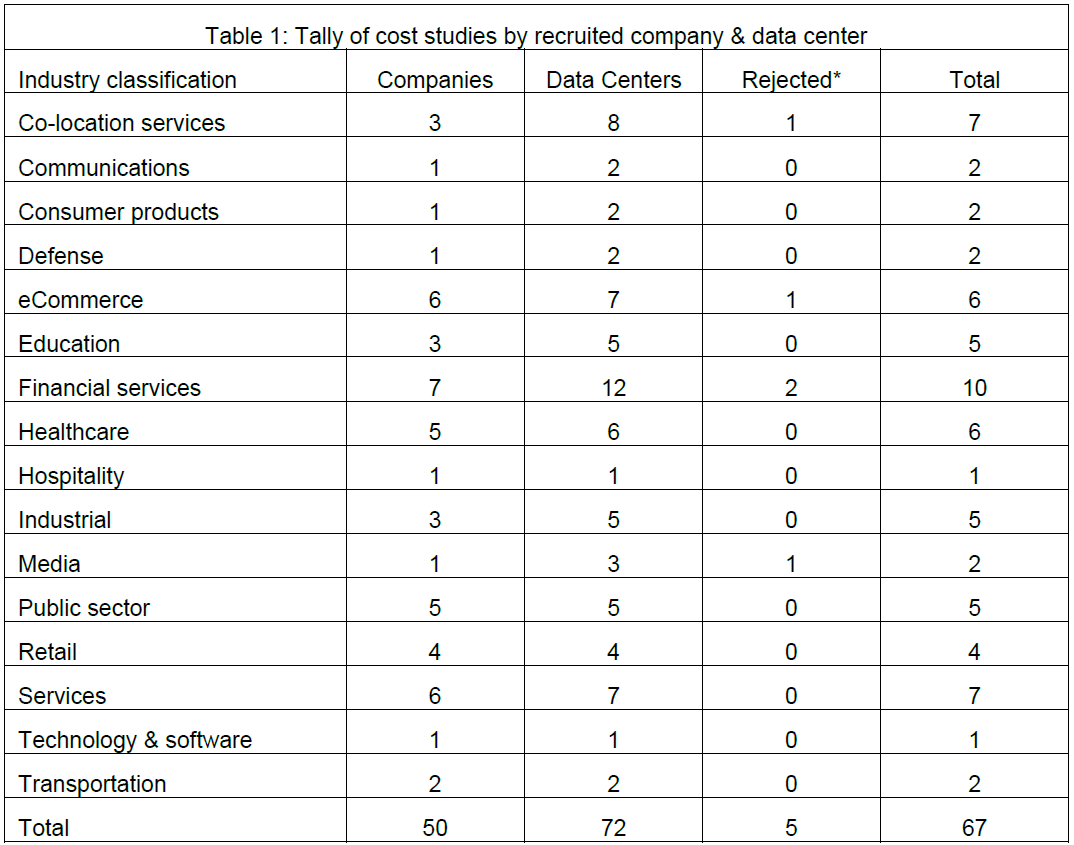
Published in: 2007 9th International Conference on Electrical Power Quality and Utilisation
Abstract
Transmission systems around the world are increasingly applying capacitor banks on their transmission systems, primarily to support transmission systems and avoid voltage collapse issues leading to blackouts. Another trend is the utilization of underground cable to obtain right of way in corridors sensitive to overhead lines. These trends both leads to harmonic resonance issues. This paper presents three separate case studies of different situations and concludes with some of the general principles that can be derived from an examination of diverse case studies.
The study of harmonic resonance issues on transmission systems is unique and difficult for a variety of reasons. First, the transmission system involves a large model that presents practical difficulties for computer simulations. Second, the transmission system can be operated under a variety of contingencies and generation dispatch that leads to different short circuit levels and impedance characteristics. Third, determining the damping affect of loads on the system is important to the results. Finally, transmission system capacitor banks are multi-staged which allows for different harmonic filter configurations, such as the C-filter.
This paper presents three separate case studies of different situations, all illustrating the unique aspects of transmission system harmonic studies as mentioned above. The case studies include the following diverse selection:
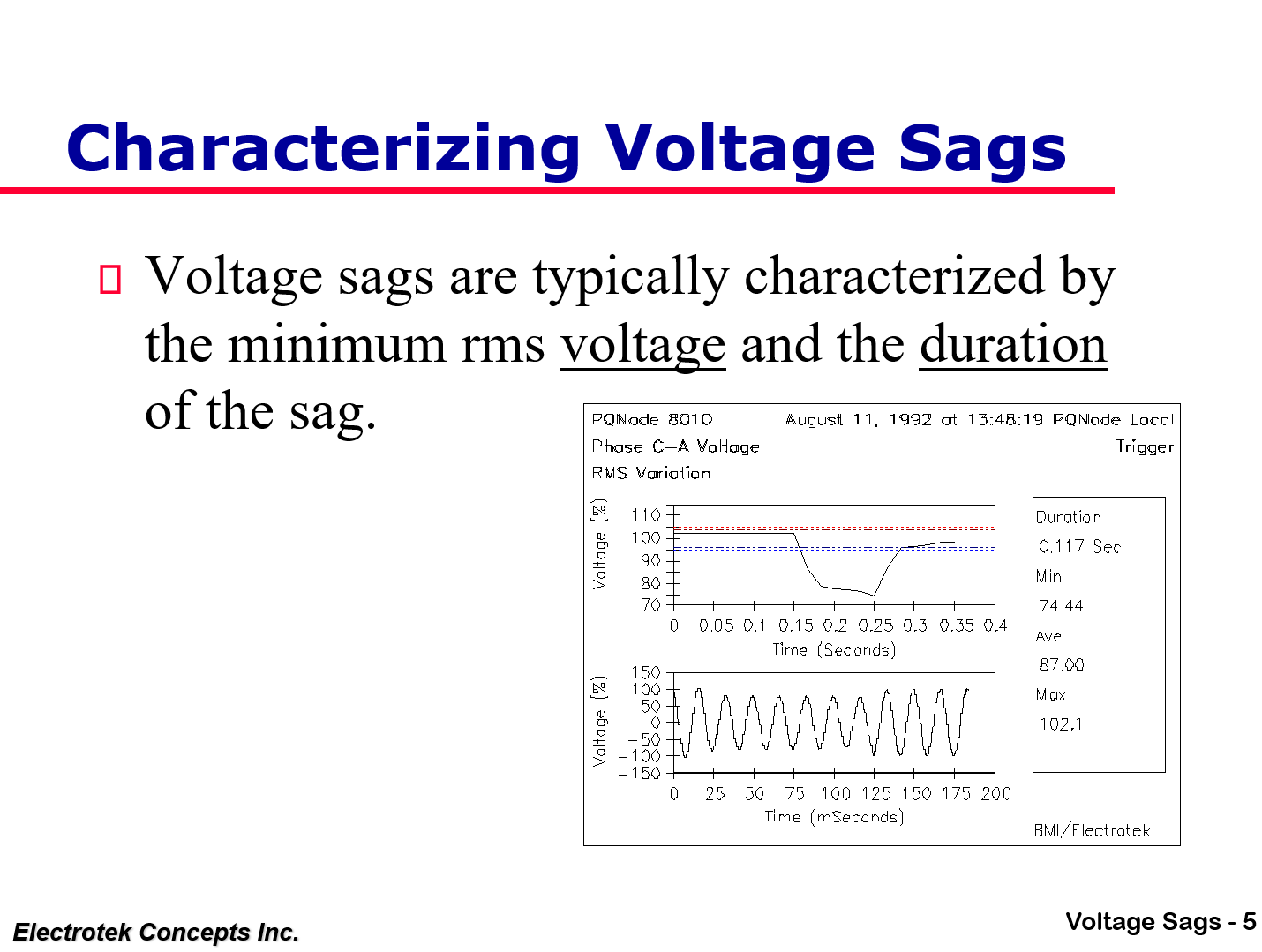
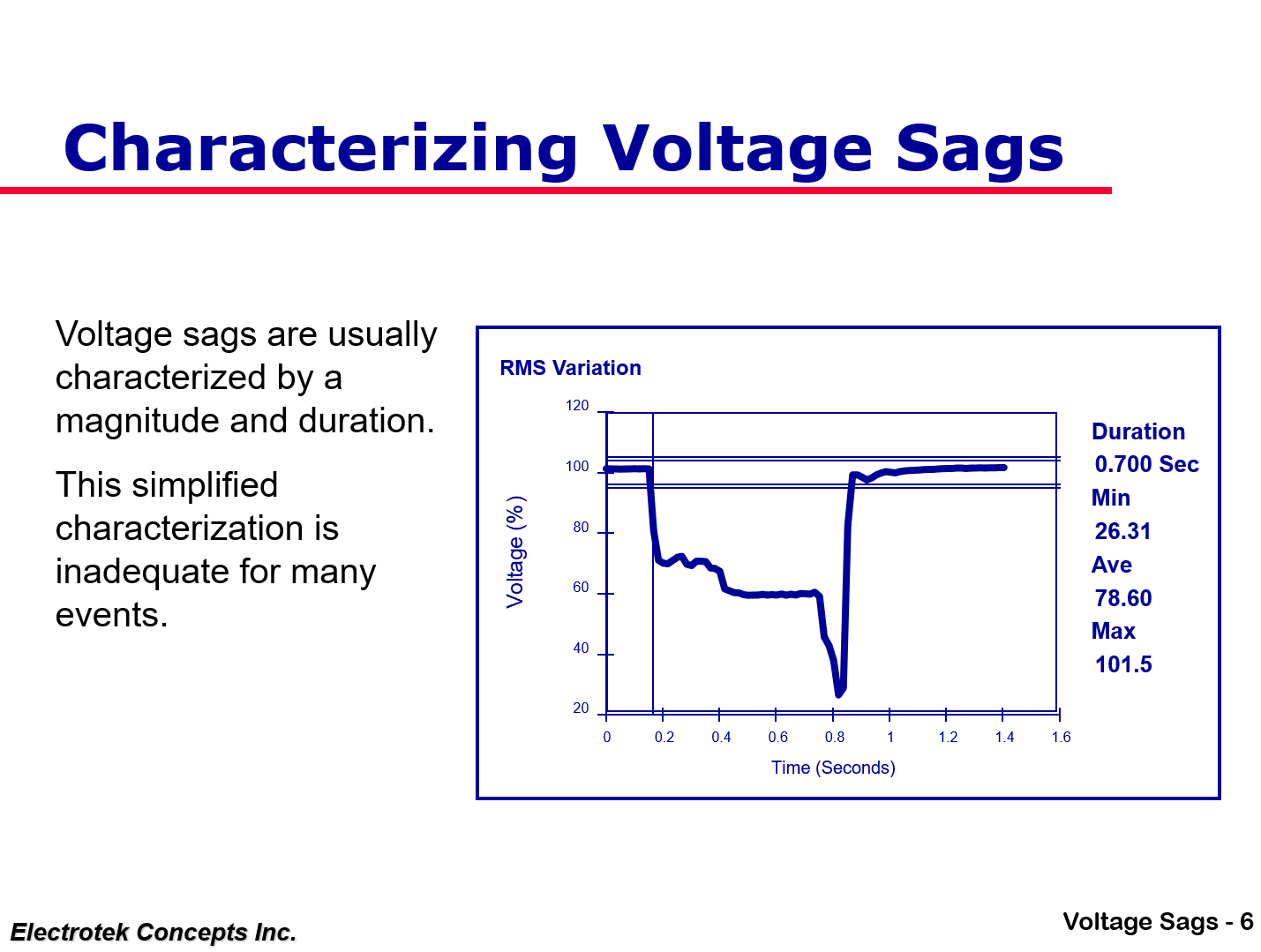
A European wind farm with an underground transmission system and its affect (under various system contingency configurations) on expected harmonic
The operation of an HVDC system in China leading to transmission system capacitor bank failures. The study shows how the cause of the problem was analyzed and how mitigation methods for the existing substation, and how that strategy might be modified for newer installations.
High harmonic voltage distortion (Vthd>10%) on a transmission capacitor bank in North America under system line outage conditions. The case includes analysis of a large network model and mitigation methods.
UNDERGROUND TRANSMISSION CONNECTION TO A WINDFARM
A windfarm under construction included 41 total turbines, each with a 2MW capacity. The site was located in a coastal area with excellent wind energy potential. The connection to the transmission system involved a new line of over 20km. Planning permission to install an overhead line was stalled; so to avoid a financial calamity the windfarm developer began planning an underground transmission line.
The transmission grid operator began studying the affects of the 20km underground transmission connector. Three-core cable has much higher capacitance than overhead line, directly as a result of much closer cable spacing. At transmission voltage levels this capacitance becomes very significant, leading to concerns for harmonic resonance.
A preliminary study by the electric utility showed that the cable did introduce harmonic resonance, particularly under a contingency of one-line out, when the resonance was near the 5th harmonic frequency. From this study the electric transmission operator was reluctant to allow the interconnection of the windfarm via the underground cable. Electrotek was hired to perform additional consulting and analysis of the situation.
Harmonic Modeling Software
The SuperHarm™ harmonics package, as developed by Electrotek Concepts, was utilized to perform all of the harmonics analysis. The software utilizes an “admittance matrix solver” approach in combination with constant current sources for harmonic generation. These afore mentioned techniques allow for a direct solution of harmonic response. The software package has been sold for over 12 years and has been extensively benchmarked with test cases for solution accuracy. Electrotek maintains a technical resource area, http://www.pqsoft.com, for users to share technical knowledge on power system simulations. Additionally, the company conducts system studies and training on harmonic analysis.
Figure 1 – Network equivalent model
Network Model
A reduced network equivalent model of the entire transmission grid system was developed as shown in Figure 1. The model included Thevenin equivalents at three different supply points, based on short circuit models and studies from the PTI/PSSE software.
The original study similarly used a reduced network for the analysis. The revised network for this later study expanded the original model, providing more detail to evaluate future network improvements and contingencies. The expanded model also allowed harmonic source equivalents to be dispersed about the network, and provided the means to evaluate the resonance concerns on nearby network locations that might have been affected by the interconnection cable or proposed harmonic solutions.
Damping Improvements
Digital computer simulations of power system phenomena at harmonics and other frequencies above nominal (50Hz) tend to present pessimistic (under damped) responses. This is because the ideal mathematical models for components such as lines, cables, transformers, and loads do not typically include enough consideration for frequency-dependant losses (such as skin effect). Generally, this concern is handled by comparing actual measurements with simulation results, and introducing damping elements to the model in order to achieve a closer comparison of the simulations with the measurements. In this particular case there is a not another cable to compare with the one being installed it is difficult to determine the appropriate amount of damping. Thusly, some conservative assumptions must be utilized, along with the consultant’s experience of other situations where some establish general guidelines.
One example of a general guideline that was utilized was the introduction of damping resistors across the Thevenin Equivalents, to provide some damping to the model at higher frequencies.
Harmonic Source Assumptions
Harmonic sources characteristics were developed from measurements taken on the network during a harmonics survey. These typical characteristics were applied at the grid substations as given in Table 1 below. Some adjustment was made on the less characteristic harmonics (3rd, 9th, 11th, 13th) to bring the predicted background levels into line with measurements that were obtained for key locations in the model.
Table 1 – Harmonic source characteristics
Harmonic Number
Magnitude (% of Load)
3
0.5 Balanced 3.0 Unbalanced
5
3.2
7
1.5
9
0.2
11
0.4
13
0.2
Frequency Scan Results
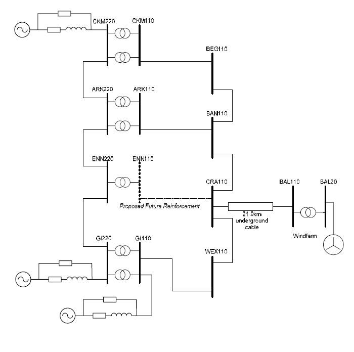
Frequency scans, or “driving point impedance” plots, are frequently used in harmonic analysis to gain physical insight into the response of the network. Figure 2 shows results from various cases, including a line out-of-service contingency that results in resonance at the 5th harmonic frequency.
Figure 2 – Frequency scans of various contingencies
Harmonic Simulation Results
Frequency scan results have limitations, particularly on transmission systems where harmonic sources may be widely distributed and there are many possible sources of resonance. A full harmonic solution case is necessary, where the harmonic voltage distortion is evaluated at all network locations. Table 2 gives some partial results of the harmonic simulations shows that distortion exceeds standard levels when the new cable is installed and especially when one line is out of service.
Table 2 – Summary of harmonic simulation results
Case
%THD
%H3
%H5
Existing
1.36
0.2
1.1
New Cable
2.39
0.3
1.7
Line 1 Out
3.08
0.2
2.5
Line 2 Out
4.14
0.7
3.9
Solutions
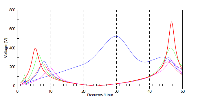
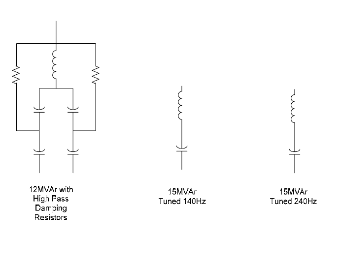
The windfarm developer was interested in providing a harmonic filter that could mitigate the problems of the new underground cable. The filter would allow the connection to be maintained (and wind power sold to the system) under contingency conditions. Figure 3 below depicts the various filter arrangements studied, including a C-Type filter. Figure 4 below gives the frequency scans comparing the various solutions.
Figure 3 – Various filter topologies investigated
Figure 4 – Frequency scans of various solution alternatives
History Description
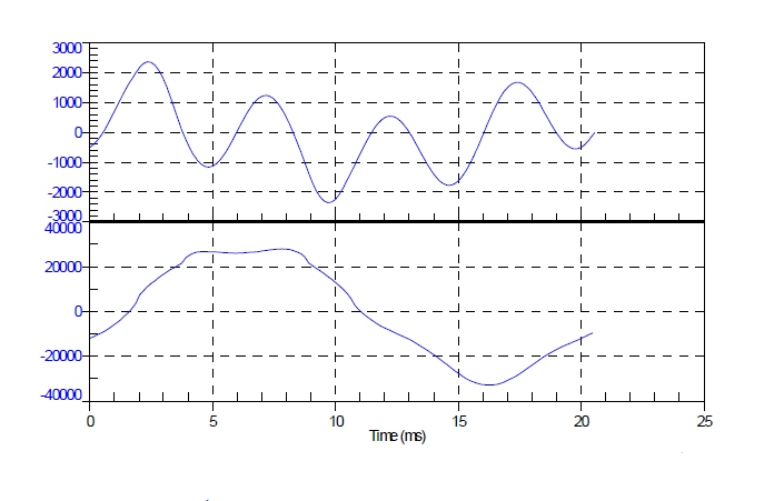
Repeated capacitor failures occurred at a tuned harmonic filter at a transmission substation, connected to the 525kV system. High levels of current were absorbed by the bank (THD=169%, Irms=200%) at the time of one of the failures. The current had an unusually high content of 4th harmonic frequency (Figure 5).
Figure 5 – Current and voltage waveform captured just prior to a failure of the bank
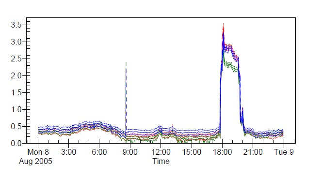
The timing of the incidents clearly identified mono-pole operation of a nearby HVDC terminal as the culprit of the failures. Figure 6 shows the trend of harmonic voltage THD at the affected substation during one of the events. DC bias, similar to that of GIC (Geomagnetic Induced Currents) phenomena, caused high transformer excitation currents rich in harmonic spectrum [1].
Figure 6 – Time trend of harmonic voltage distortion
System Description
The substation was connected to the 525/242kV system with a 750MVA autotransformer with a 34.5kV tertiary. The 34.5kV busbar supplied reactive compensation consists of three main units on the 34.5kV bus:
40.08MVAr, 41.57kVAr, 16.5mH (144Hz)
40.08MVAr, 38.11kVAr, 5.8mH (223Hz)
40.08MVAr, 38.11kVAr, 5.8mH (223Hz)
These units were initially designed to provide reactive power compensation while avoiding problems at characteristic (i.e. 3rd, 5th, 7th) harmonic frequencies, and also to minimize transient switching concerns. They were properly sized with higher voltage ratings to accommodate the voltage rise through the reactors.
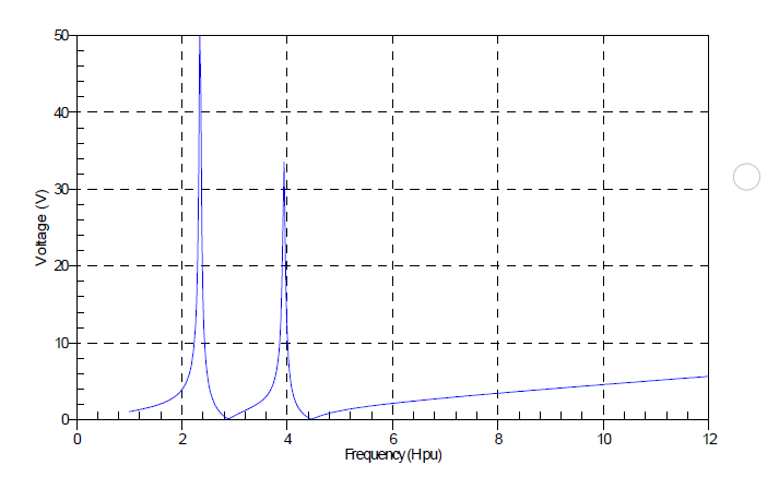
Figure 7 – Frequency scan at the 34.5kV bus
Harmonic Simulation Results
Harmonic simulations confirmed that the configuration of the capacitor banks as harmonic filters results in a series resonant condition at the 4th harmonic frequency (Figure 7), where the bank absorbs excessive 4th harmonic current. During normal conditions there are very few sources of fourth harmonic current. However, during the monopole operation of the HVDC terminal the DC bias results in high transformer excitation current, rich in 4th harmonic content (Table 3).
Table 3 – Transformer full load current under DC bias
H
Magnitude
1
825.213
2
212.198
3
141.465
4
94.3101
5
35.3663
Figure 8 shows the simulation results for the waveforms of the voltage and currents (144Hz and 223Hz tuned units). The results show that even with just one transformer in DC bias (and the effect likely involved other units) the filter tuned near the fifth harmonic will absorb a high amount of fourth harmonic current.
Figure 8 – Simulation results for the 34.5kV bus
Solution
Simulations confirmed that the reconfiguration of the capacitor banks, either tuning all banks to 144Hz, or reconfiguring as C-Type filters would resolve this problem. For future banks it is probable that the 144Hz configuration is best although this requires higher voltage rated capacitors. For the existing bank it is easiest to reconfigure as a C-Type filter, as the existing capacitor bank can be reconfigured.
CAPACITOR BANK RESONANCE IN THE USA
Case History Description
Four identical 52.8MVAr capacitor banks are installed at a transmission substation serving a large city on separate and distinct buses that are numbered 1, 2, 3, and 4. During normal operation of the two banks on buses 2 and 4, voltage total harmonic distortion (THDv) was seen to range about 4-5%. While these levels are probably acceptable for short term operation, they exceed the recommended limits of the IEEE- 519 Standard [2] for harmonics as shown in Table 4 below.
Table 4 – IEEE-519 harmonic voltage limits
Bus Voltage
Maximum Individual Harmonic Component
Maximum THD
69kV and below
3.0%
5.0%
115kV to 161kV
1.5%
2.5%
Above 161kV
1%
1.5%
No appreciable harmonic distortion issues were detected from the operation of banks 1 and 3. A comparison in Table 5 of the available short circuit levels at the substation shows that banks 1 and 3 have a higher fault current availability and so they are less likely to cause harmonic resonance concerns.
Table 5 – Available fault levels at the substation
Bus
3 Phase MVAsc
52.8MVAr H resonant
1
4762
9.5
2
3189
7.8
3
4490
9.2
4
3117
7.7
Later, when the banks 2 and 4 were operated during a lineout contingency harmonic voltage distortion levels (THDv) of about 10% were experienced. At the same time the current harmonic distortion in the capacitor bank exceeded 50%. These levels of harmonic distortion are clearly detrimental to power quality, and should be avoided for all but the briefest periods of time (minutes). Also the nearby distribution substation experienced some nuisance tripping of protective devices.
The prudent step of reducing the size of Banks 2 and 4 was done by reducing one (of four) strings of parallel capacitor arrangements, derating the size of the bank to 39.6MVAr. A harmonic study of the situation was undertaken.
System Model
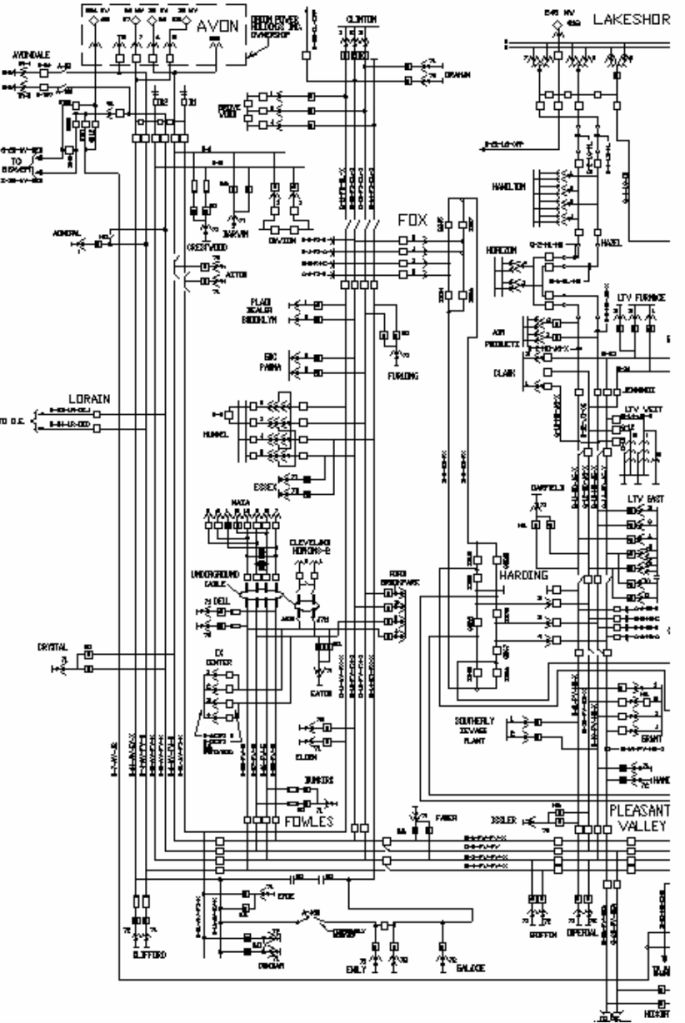
A fairly extensive transmission system network was used for the study. The figure below represents the part of the network that was included in the study. In the end the model included over 900 buses. As capacitor banks for reactive power compensation were distributed about the transmission system, it was necessary to develop such a large model. Impedance data for the model was imported from the short circuit model of the network and facilitated by spreadsheets and batch files. Every three-winding transformer of the system had to be checked against the original test reports, as the impedance values did not always transfer properly through the short circuit program.
Figure 9 – Partial diagram of the system modeled
Simulation Techniques
Loading information from various system buses was used to inject harmonic sources. Table 6 gives the harmonic source characteristics that were used as a percentage of the load. The harmonic source characteristics were adjusted to obtain agreement with available harmonic measurements.
The system supplies some very large industrial loads that contribute a relatively high percentage of harmonic loads. Ideally the largest industrial loads would be characterized for their harmonic content, but such detailed measurements were not available.
Table 6 – Harmonic source characteristics
Harmonic Number
Magnitude (% of Load)
3
0.5
5
8.0
7
3.0
9
0.3
11
1.5
13
1.0
Figure 10 depicts a list of simulation cases where various capacitor banks were in/out of service. Both frequency scans and simulation cases were run with the various configurations. These results allowed insight into the effects of different units. Some units would introduce objectionable resonance, other units would tend to alleviate problems by shifting resonance conditions.
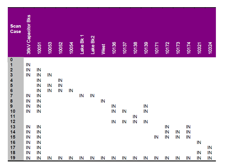
Figure 10 – Case list of simulations
One factor critical to the analysis was considering contingency conditions, when various lines would be out of service. Lines going to substations with major capacitor banks are very important, as the fault level is often greatly reduced. This in turn affects resonant frequency, and is often a limiting factor in the design of the capacitor bank.
Study Results
Banks 1 and 3 have a strong enough supply that they are not expected to cause any harmonics problems. Even during one-line-out contingencies, the source is strong enough to avoid problems at the 5th or 7th harmonic frequencies.
Various frequency scans given the report showed that Buses 1 and 3 are affected by the operation of certain other capacitor banks, but not all of them. Many times these effects occurred at the 11th and 13th harmonic frequencies and were not found to create operational issues.
The distribution system had 36kV capacitor banks that were modeled in this study. In this particular case they were found to have little effect on the results. However, in a subsequent study of a different network area, distribution capacitor banks were found to have an important mitigating effect.
Some problems were encountered as some of the simulation results did not match well with the measurement results. Particularly on bus 4, it was found that the fault levels reflected contributions from large industrial motors and generators that were not always in service. The fault levels in the model were deemed to be higher than those actually available during the measurements. When some adjustments were made for these realistic conditions, the results matched more closely.
CONCLUSION
The study of harmonic resonance issues on transmission systems is unique and difficult for a variety of reasons. First, the transmission system involves a large model that presents practical difficulties for computer simulations. Second, the transmission system can be operated under a variety of contingencies and generation dispatch that leads to different short circuit levels. Determining the damping affect of loads on the system is important to the results. Finally, transmission system capacitor banks are multi-staged which allows for different harmonic filter configurations, such as the C-filter.
REFERENCES
[1] R.A. Walling, A.H. Khan; “Characteristics of transformer exciting current during geomagnetic disturbances”, IEEE Transactions on Power Delivery, Vol. 6, No. 4, October 1991.
[2] IEEE 519 “Recommended Practices and Requirements for Harmonic Control in Electric Power Systems” 1992.
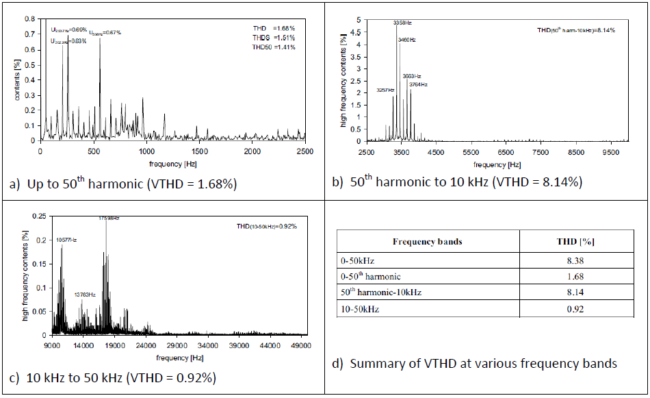
Trademarked flex CT interface WideRangeFlexCT™ measures currents from 1A to 2500A without requiring the user to set specific ranges. Internally there are 3 measurement ranges that are automatically switched between.
The measurement error depends on which range is active, these ranges are 1.00A – 18.00A, 18.0A – 180.0A and 180A – 2500A.
The total measurement error will depend on different factors: the component tolerances of the electronic interface, the manufacturing tolerances of the flex CT coil and the position of the flex CT with respect to the conductor. For minimum positional error, the ideal position is for the flex CT loop to be perpendicular to the conductor with the conductor passing through the center of the loop. In field installations it is difficult to ensure that the conductor passes through the center of the loop, so we calibrate the flex CTs with the conductor passing perpendicular through the loop but positioned on the edge of the loop at the farthest point from the flex connector.
With the conductor positioned the same as during calibration the measurement errors are:
1.00A – 18.00A: ± (0.02A + 0.5% of reading)
18.0A – 180.0A: ± (0.2A + 0.5% of reading)
180A – 2500A: ± (2A + 0.5% of reading)
Non-ideal positioning can add an additional 1% of reading error.
Limited resources or need a solution quickly?
If you need additional information about your project just contact us, we are here to help. We can support you at any level from telephone support, or on-site solutions for a reasonable price.
Contact us at radian@radianresearch.com or call 765-449-5500. Be assured that we want to be your partner in success!
Earth resistance is a key parameter in determining the efficiency of earthing systems. In this article we look at the measurement of earth resistance
1 A Few Fundamentals
1.1Earth resistance and earth impedance
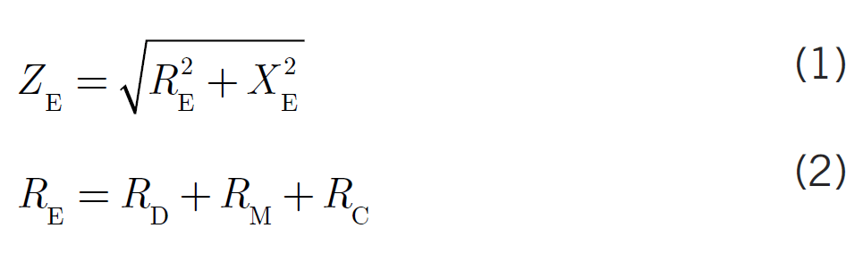
The efficiency of an earthing system is principally determined by its impedance ZE. As can be seen from figure 1, the earth impedance can be expressed as in equation (1):
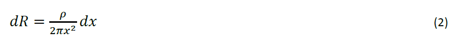
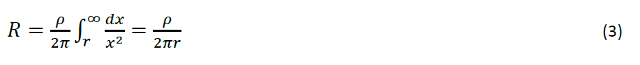
As shown in equation (2), the earth resistance RE is the sum of the dissipation resistance RD, the resistance of the metal conductor that serves as the earth electrode RM and the resistance of the earthing conductor RC, which runs between the main earthing busbar and the earth electrode. The dissipation resistance RD is the resistance between the earth electrode and the surrounding soil. The reactance of the earthing system XE can be expressed as:
with XM reactance of the metallic earth electrode XC reactance of the earthing conductor.
For AC supply current the reactance of the earthing conductor is only significant in the case of extended horizontal earthing strips or long earth rods. In all other cases, the difference between earth impedance and earth resistance is so small that frequently no distinction is made between these two quantities. The relevant industrial standards also treat earth impedance and earth resistance as identical.
As earthing measurements are carried out using an AC supply, it is actually the earth impedance that is measured. If the measurement frequency is greater than 50 Hz, a slightly larger earth impedance is displayed. However, overestimating the earth impedance is not a problem, as it errs on the side of safety.
Figure 1Vector diagram of impedance in an earthing system
RD dissipation resistance; RE resistance of the earthing system (earth resistance); RM resistance of the metal conductor that acts as the earth electrode; RC resistance of the earthing conductor (e.g. connection lug, cable); XE reactance of the earthing system; XM reactance of the metal conductor that acts as the earth electrode; XC reactance of the earthing conductor; ZE earth impedance; ϕ impedance angle.
1.2 Requirements for earthing measurements
Earthing measurements are necessary whenever compliance with a specified earth resistance or a particular earth impedance is required, as is the case in the following earthing systems:
Protective earth for TT and IT earthing systems low-voltage installations ([1], sections 411.5 and 411.6; [2]);
Joint earthing system for high-voltage protective earthing and functional earthing in transformer substations;
Earthing system for the neutral earthing reactor of a medium-voltage distribution system.
In the case of lightning protection systems, earthing measurements must be made even when there is no requirement to comply with a specific value. The results of repeat tests must be compared with those of earlier measurements.
1.3Standards for measuring instruments
The standards contain the requirements that have to be met by the manufacturers of measuring equipment. For users, these standards serve only informational purposes.
In low-voltage systems earthing measurements must be made using equipment that complies with the VDE 0413 standards (VDE: Verband der Elektrotechnik Elektronik Informationstechnik e.V./ engl.: Association for Electrical, Electronic & Information Technologies) (see [3], sec. 61.1). All equipment must comply with the specifications in IEC 61557-1:2007 [4]. In addition, equipment must also comply with the following standards depending on the type of device or measuring method for which it is used:
IEC 61557-5:2007 Equipment for measuring resistance to earth [5]
IEC 61557-6:2007 Equipment for testing, measuring or monitoring protective measures involving residual current devices [6]
Equipment manufactured in accordance with earlier editions of the VDE 0413 series of standards can of course also be used.
1.4Selecting the right measuring equipment
It is not enough for users to simply follow the (frequently unclear) instructions provided by the manufacturer, they need to be aware of and understand the measuring method they want to apply. Measuring instruments that do not make it clear which measuring method is being applied should not be used.
Before purchasing equipment, users should request technical descriptions of the devices of interest as well as their performance data and, if possible, instruction manuals, and should assess the equipment on the basis of this documentation.
1.5Avoiding hazards and measuring errors
The process of measurement and any accompanying procedures (e.g. breaking standard connections and making non-standard connections) must not pose a safety hazard ([3], sec. 61.1.3). The magnitude of the test voltage or the test current must be limited (see sections 3.1 and 4.1). Before breaking a connection that is required for electric shock prevention, the entire power installation must be disconnected from the supply and locked out to prevent it being switched on again.
Any measurement that involves breaking connections (e.g. opening the inspection joint of a lightning protection system) must never be carried out during a storm or whenever a storm could be expected. Failure to comply could be hazardous, particularly for the person performing the operation. After the measurement has been completed, any connections that were broken must be properly restored.
If the test current is split so that part of it runs parallel to the earth electrode being measured, the earth resistance displayed by the meter will be too small. The person conducting the measurement must therefore be aware of everything that is connected to the earth electrode under test [8]. Measurements must only be carried out by competent persons.
1.6Taking the effects of weather into account
The specific resistance of soil decreases with increasing temperature and increasing soil moisture levels. Whereas these effects are of minor consequence for foundation earth electrodes in buildings with a basement or for long (vertical) rod electrodes, they have to be taken into account in the case of horizontal surface earth electrodes.
Measurements made during cold, dry weather remain unaffected, but measurement data recorded in warm weather or after a rain shower have to be adjusted upward.
1.7Assessing measurement results
Earth resistance meters are not error free. Measurement errors can occur even if the conditions specified in the relevant standards and instrument instruction manuals are complied with and even in the absence of interference effects. The magnitude of an instrument’s operating error is listed on its technical specification sheet or in its instruction manual. In those methods of measuring earth resistance that draw current directly from the power source (see sections 2.4 and 4), additional measurement uncertainty can be caused by random current and voltage fluctuations in the supply during the measurement.
Examples of possible operator errors include:
failure to take account of connections detrimental to the measurement process
connecting the instrument leads incorrectly or selecting the wrong setting on the selector switch of the instrument
inserting the auxiliary earth electrode or probe in the wrong location
meter reading errors
failure to implement measures to reduce systematic measurement errors.
Results from first-time measurements should be compared with the project specifications, results of repeat tests should be compared with those of earlier measurements. If significant differences are apparent, the possible causes of the discrepancy should be determined. The influence of weather on the measurement results and how this can be taken into account is discussed in section 1.6.
1.8Test report
Measuring earth resistance is only one of several tests that have to be performed on earthing systems [9]. In general, the results from all the tests are contained in a single test report. The measurements performed and any accompanying action that is taken must be described precisely so that they can be reproduced at a later date. Information that must be provided includes:
the measurement method used
the type of measuring instrument used
the positions of any selector switches, if relevant
details of any connections that were broken or made for the purposes of the measurement.
The results of the measurement must be stated clearly and unambiguously. This also applies to any weather-related adjustments of the results that may have been made.
The test report is required by
[3], section 61.1.6 concerning earthing systems in low-voltage networks
[10], annex E, section E.7.2.5 concerning lightning protection systems
both standards apply if the earthing system serves both purposes.
2Overview of Measurement Methods for RE
2.1Principles
There is a wide degree of variation in the internal circuitry of the measuring instruments used and the layout and arrangement of the external measuring circuits. However, a common feature of all the methods is that they determine the earth impedance by measuring the voltage across the earthing system for a known test current. Leads that carry the test current outside of the instrument are shown in red in the diagrams.
Known measurement methods are listed in table 1. The underlying circuit principles are shown in figures 2 to 4. The unusually long names given here to the various methods ensure that the methods can be distinguished unambiguously.
Although there are clear differences between the individual measurement methods, no one particular method can be said to be ideal. Each method has its own particular disadvantages such as limited applicability, electric shock hazard, larger measurement errors or requiring greater time and effort to complete. The various advantages and disadvantages of the individual measurement techniques are described in more detail in sections 3 and 4. All of the methods discussed must only be carried out by competent persons exercising due care and attention. In those methods that do not draw current directly from the supply (columns 1 to 6 in table 1), the measurement frequency used will be at least 5 Hz above or below the frequencies 16.7 Hz, 50 Hz and integer multiples thereof. This prevents interference from supply frequency currents (‘interference currents’) that can falsify measurement results.
In those methods that do draw current directly from the supply (columns 7 to 9 in table 1), it is of course essential that the supply frequency and measuring frequency are identical. This means that the interference effects mentioned above cannot be ruled out when such methods are used. However, these methods are simpler to perform and offer advantages in terms of their applicability.
Table 1 Overview of earth resistance measuring methods
2.2The balanced-bridge method
The balanced-bridge method as described by Behrend is one of the techniques for measuring earth resistance that does not involve drawing current directly from supply. Earth resistance meters based on this method are no longer manufactured, as other more user-friendly instruments have now been developed for the same sorts of applications. These new meters use the so-called current-voltage method, which also does not involve current being drawn from the supply. Nevertheless the balanced-bridge method is described here because it is of fundamental importance to the development of earth resistance measurement techniques and because meters based on this method are still in use.
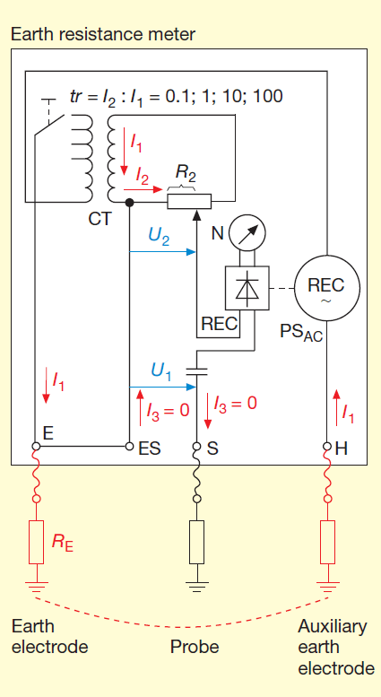
The measurement circuit for the balanced-bridge method is shown in figure 2. The method involves driving an auxiliary earth electrode1) and a probe2) temporarily into the soil. When the earth meter is in its balanced state, there is no current flowing in the probe. The resistance to earth of the probe has therefore no influence on the measurement result; it simply lowers measurement sensitivity. Information on the alignment and separation of the auxiliary earth electrode and the probe is provided in section 3.
The AC power source PSAC is located between the connection point for the earth electrode under test (socket E) and that for the auxiliary earth electrode (socket H). The AC source is connected in series with the primary winding of a current transformer CT. Connected to the secondary winding of the current transformer is a variable voltage divider. The setting chosen for the left part of the divider R2 (‘reference resistance’) is displayed on the scale on the voltage divider’s control unit. A null detector N with a rectifier REC in series is located between the variable tap point of the voltage divider and the connection point for the probe (socket S). The rectifier is driven by the AC power source. A capacitor C prevents any DC current from flowing across the probe. One end of the voltage divider is connected to the earth electrode being measured via the instrument sockets ES and E. The transformation ratio tr of the current transformer can be switched to achieve the required measurement range.
When balanced, the current I3 in the probe is zero. The same current I1 therefore flows in the auxiliary earth electrode and in the earth electrode under test. Additionally, the voltages U2 (‘reference voltage’) and U1 are of the same size. The voltage U1 corresponds to the earth electrode voltage that drives the test current I1 in the earth resistance RE of the test object E, whereas U2 is the voltage drop that maintains the current I2 (‘reference current’) in the reference resistor R2. The potential drops obey Ohm’s law as expressed by the equations U1=I1 · RE and U2=I2 · R2. If the transformation ratio of the current transformer tr = 1:1, then I2 = I1 and the value of the earth resistance RE is equal to the selected reference resistance R2. The earth resistance can therefore be read off the voltage divider scale mentioned above. If another transformation ratio is used, this must be multiplied by the value of the reference resistance R2, i. e. RE=tr ·R2.
Figure 2: The balanced-bridge method
REC rectifier; I1 test (or measuring) current; I2 Reference current; I3 current whose magnitude is zero when bridge is balanced; C capacitor; N null detector; RE earth resistance being measured; R2 reference resistance; CT current transformer; U1 Voltage across earth electrode under test; U2 reference voltage; tr transformation ratio of the CT; PSAC AC power supply.
2.3 Other measurement methods without supply current
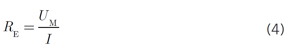
Another group of methods for measuring earth resistance that do not draw current directly from the supply are the so-called current-voltage techniques illustrated in figure 3. The earth resistance RE is determined from the voltage UM that appears across the earth electrode and across the sockets ES and S, and the measured current I.
Figure 3 simply illustrates the principle of the measurement and shows only a small part of the complex circuitry within the earth resistance meter. Usually, the voltage UM and current I are not shown separately and the meter only displays a digital reading of the earth resistance RE. If the AC supply source PSAC is a constant-current generator, the earth resistance can be displayed directly on the voltage meter. When the balanced-bridge method was first developed, the only exterior circuit known was that shown in figures 2 and 3a). It was therefore usual to consider the circuitry inside the meter and the exterior circuit as a single entity. However, as indicated in columns 2 and 3 in table 1, the same meter can be used for measurements with the exterior circuits shown in figures 3b) and 3c). Equally, the earth resistance meters used for the current-voltage methods that do not draw current directly from the supply can be used like the meters designed with the balanced-bridge circuit. The internal circuits can therefore be freely combined with the exterior circuits.
Figure 3 Current-voltage methods that do not draw current directly from the power supply
a) with probe and auxiliary electrode;
b) with probe, but without an auxiliary electrode;
c) no probe, no auxiliary electrode (measures resistance of conductor loop via earth return path). I test current; Rloop loop resistance; UM test voltage.
Figure 4 Current-voltage methods that draw current directly from the power supply
a) with probe;
b) using PEN conductor or neutral conductor instead of probe;
c) no probe (measures resistance of conductor loop via earth return path); U0 conductor-to-earth voltage
2.4Measurement methods with current from the supply
These methods can only be used in networks with a direct connection to earth. As shown in figure 4, the measurement involves drawing the test current from the phase conductor of the supply system. The meters used in this type of measurement are primarily designed for testing electrical safety systems involving residual current devices. The meters are generally connected to the supply via a flexible power lead and an earthed safety plug.
3Current-Voltage Method that Draws No Supply Current
3.1Earth resistance meters
The four connection sockets are labelled as shown in figure 5. Sockets for the supply current path and for current measurement:
E – Earth electrode (test object)
H – Auxiliary earth electrode1) Sockets for the voltage measurement path:
ES – Earth electrode (or the probe located close to the earth electrode when measuring the soil resistivity)
S – Probe2) Normally when measuring the resistance to earth, the sockets E and ES are connected to one another via a removable link or via a contact strip within the meter’s selector switch as this ensures that the earth electrode under test is connected to both the current and voltage measurement paths. If, in addition, a jumper is placed between sockets H and S, the earth resistance meter can be used as a simple ohmmeter.
The frequency of the AC supply PSAC is at least 5 Hz above or below the frequencies 16.7 Hz and 50 Hz and any integer multiples thereof. Typically, the supply frequency is in the range 41–140 Hz, though in some meters a higher frequency is used. Some earth resistance meters also offer the option of selecting the frequency. A number of meters with automatic frequency control (AFC) automatically switch to that frequency offering the lowest level of interference.
To protect against electric shocks, the open-circuit test voltage generated by the meter must not exceed 50 V (r.m.s.) and 70 V (peak). In the case of earth resistance meters used on agricultural sites, these values must be halved. Alternatively, the short-circuit current must not exceed 3.5 mA r.m.s. and a peak value of 5 mA (see [5], sec. 4.5). If neither of these conditions are met, the meter must switch off automatically.
The meter is powered either by a battery, a group of primary cells or a hand-driven generator, though the latter method is now rare. The meter must indicate whether the end-point voltage of the power supply is sufficient to maintain proper instrument function (see [4], sec. 4.3).
When earth resistance is measured by a method that does not involve current being drawn directly from the supply, the earth resistance RE is computed as the quotient of the measured voltage UM that appears across the earth electrode (and across the meter sockets ES and S) and the measured current I (that flows through sockets E and H). Figure 5 only indicates the basic principle of the complex circuitry within the meter. Usually, the voltage UM and current I are not shown separately and the meter only displays a digital reading of the earth resistance RE. If the AC supply source is a constant-current generator, there is no need to measure the current and calculate the quotient. In this case a voltage meter can be calibrated to display the earth resistance directly.
Most meters are equipped with a switch for selecting the type of measuring circuit, the measurement frequency and/or the measurement range, and for switching the power on and off. Most meters also have a button that is used to initiate measurement. The earth resistance meter must also indicate that the resistance of the auxiliary earth electrode and the probe are within the specified limits (see [5], sec. 4.4). However, it is not advisable to rely too heavily on a warning signal, because by the time a warning signal has been issued, the limit may have been exceeded by a significant amount. User-friendly devices offer additional functions such as:
warning signal or automatic cut-out if too great an interference voltage is detected
warning signal or disabling of measurement function if test current is too small
display of test current (for monitoring purposes only when measurements made with a constant-current generator)
automatic measurement range selection
display hold function
data storage for transmitting or printing measurement results.
Figure 5 Current-voltage methods that do not draw current directly from the power supply and that use a probe and an auxiliary earth electrode
I test current; RE earth resistance being measured; RE´ measured earth resistance; UM test voltage
3.2 Methods Using a Probe and An Auxiliary Earth Electrode
3.2.1 Principle
As shown in figure OE, the earth electrode under test, an auxiliary earth electrode and the probe are connected to the earth resistance meter. The test current I flows through the earth electrode, the soil and the auxiliary earth electrode. The voltage UM that appears across the earth resistance RE also appears across the meter sockets ES and S. The earth resistance is displayed as the value of UM divided by I.
3.2.2Earth electrode (test object)
If socket E is connected to the beginning of the earthing conductor (at the main earthing terminal), the earthing conductor will be included in the measurement of the earth resistance. If, on the other hand, socket E is connected directly to the earth electrode, the resistance of the earthing conductor will not be included in the measurement. The difference, however, is usually slight.
The resistance of the measuring leads will be included in the measurement. This will result in an overestimation of the earth resistance and thus yield a value that errs on the side of safety. To reduce the magnitude of the error, it is expedient to position the earth resistance meter close to the point of connection and to use a short measuring lead. The resistance of the measuring lead can of course be measured and this value subtracted from the value displayed by the earth resistance meter. If the effect of the measuring lead’s resistance is to be avoided at all costs, the jumper linking sockets E and the ES must be removed and each socket connected to the earthing system by its own measuring lead.
The earth electrode under test must not be connected to any other earth electrodes as this would falsify the result of the measurement. In the TN earthing systems found in consumer installations, the earthing conductor must be disconnected from the main earthing busbar as the latter is connected to the PEN conductor of the supply network. This is not required in TT systems as the main earthing busbar is not connected to the neutral conductor of the power supply network. If, nevertheless, the earthing conductor is disconnected, the entire system must be de-energized beforehand and locked out to prevent it being switched on again.
3.2.3Auxiliary electrode1)
The auxiliary earth electrode should be positioned as far away as possible from the earth electrode under test, so as to minimize the degree of overlap between the potential gradient areas (‘spheres of influence’) surrounding the two electrodes. The larger the electrodes, the farther apart they must be. As a rough guide, the minimum distance apart can be taken to be three times the depth of a rod earth electrode or the average diameter of a ring earth electrode. The figure of 40 m that is found in the documentation provided by some manufacturers can only be considered to be a rough average value. Whether the chosen distance is appropriate will be shown when the correct alignment and positioning of the electrodes is carried out (see sec. 3.2.4).
The greater the resistivity of the soil, the longer the auxiliary electrode needs to be and the deeper it needs to be driven into the ground. If the resistance of the auxiliary earth electrode is too large, measurement errors can arise, because, for example, the constant current normally generated by the AC supply cannot then flow. In such cases, it can prove useful to saturate the area of ground being used for the measurement with water.
3.2.4Probe2)
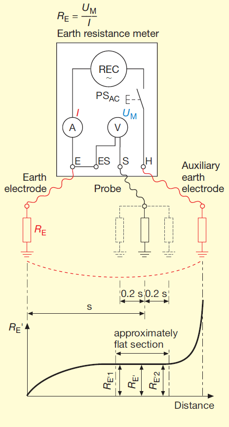
As the internal resistance of the voltage measurement path is very large, the resistance of the probe and therefore the size of the probe is of minor importance. The preferred location of the probe is on the straight line between the earth electrode and the auxiliary earth electrode at a position where it has minimum interaction with the spheres of influence of the two electrodes (see diagram in figure 5).
If one were to carry out a series of measurements with different distances between the earth electrode and the probe the results would form a curve whose ends are relatively steep while the intermediate section of the curve is flatter. If the distance between the earth electrode and the auxiliary electrode is large enough, the curve will have an approximately horizontal central section in which the measured resistance to earth is essentially independent of electrode separation.
This central section must be determined by at least three measurements. The midpoint of the central section is not midway between the earth electrode and the auxiliary earth electrode, but lies closer to the auxiliary earth electrode as the spatial extent of the spheres of influence associated with the two earth electrodes differ. In general, the optimum separation between the earth electrode and the probe is about two thirds of the distance between the earth electrode and the auxiliary earth electrode3).
3.2.5Limitations of method
If no portion of the resistance vs. distance curve is approximately horizontal, then the distance between the earth electrode under test and the auxiliary earth electrode is too small. If the curve exhibits an unusual profile, buried metal installations (e. g. water pipes) are very probably influencing the measurement. In such conditions it is not possible to achieve usable results from the measurement. Measurement may be possible if the electrodes can be laid out perpendicular to their original direction or perpendicular to the longitudinal axis of the buried metal installation or so that they run away from and not above the buried metal installation.
It is also not possible to achieve reliable results if the earth electrode under test is surrounded by other earth electrodes, for example in areas with a high density of buildings. Furthermore measurement is impossible whenever the auxiliary earth electrode and the probe cannot be positioned in the right locations. In all such cases, another measurement technique must be selected.
1) In some publications the auxiliary electrode is also referred to as the outer test electrode, or current test stake. 2) In some publications the probe is also referred to as the inner test electrode, or voltage test stake. 3) Some manufacturers state that the distance between the earth electrode and the probe should be half the distance between the earth electrode and the auxiliary earth electrode. That is incorrect. Other companies recommend placing the probe at a distance from the earth electrode that is always 62 % of the separation between the earth and the auxiliary earth electrode. This method is thus sometimes referred to as the 62 % method. The 62 % mark generally gives a good approximation of the correct location. But the optimum position must always be determined by moving the probe to neighbouring positions.
3.3Method Using a Probe But No Auxiliary Earth Electrode
3.3.1Principle
As shown in figure 6, the functional earth of the supply network acts as a replacement for the auxiliary earth electrode. It is extremely important to ensure that the connection is not accidentally made to one of the phase conductors.
In a TN system, the H socket of the meter has to be connected (for instance, via the earthing contact of a plug) to the protective earth (PE) conductor, which itself has been branched off the PEN conductor. The meter socket E is connected to the earthing conductor, which has to be disconnected from the main earthing busbar. Supply networks configured with the TT earthing system have a neutral conductor instead of the PEN conductor. This has to be treated as a live conductor even though it is connected to a functional earth. Applying this method of measuring earth resistance to a TT system would therefore involve connecting the earth resistance meter to the neutral conductor. The method is therefore not approved for use with TT systems.
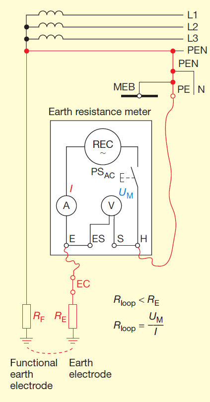
Figure 6 Current-voltage methods that do not draw current directly from the power supply and that use a probe but no auxiliary earth electrode
EC earthing conductor; MEB main earthing busbar; RB resistance to earth of the functional earth electrode
3.3.2Problems in the TN system
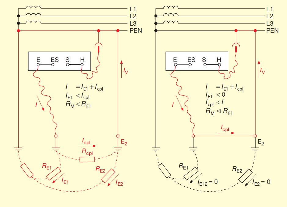
The method does not function in a TN system if the electrode being measured is strongly coupled or if it is connected via a metal conductor to another earth electrode that itself is connected to the PEN conductor. This would result in the test current flowing in the wrong path so that the display on the earth resistance meter would be smaller than the true value of the resistance to earth. This is discussed in more detail in section 3.4.2.
3.4Method Without a Probe and an Auxiliary Earth Electrode (‘Stakeless Method’)
3.4.1Principle
This method (illustrated in figure 7) is an earth-loop resistance measurement because it involves measuring the resistance of a conductor loop via an earth return path. The S and H sockets of the earth resistance meter are connected together. The advantage of this method is that neither an auxiliary earth electrode nor a probe need to be used.
In a TN system the earthing conductor (EC) is disconnected from the main earthing busbar (MEB) and the earth resistance meter is inserted between them. This method is not suitable for measurements on a consumer installations with a TT earthing system.
The resistance measurement displayed on the meter includes the resistance to earth of the functional earth and the resistance of the PEN conductor. If they were accurately known, these values could be subtracted from the resistance displayed on the meter. However, they are difficult to determine, because the functional earth in a TN system comprises not only the functional earth electrode shown in figure 7, it is also connected to numerous earths in the consumer installations of neighbouring buildings. The error that is introduced by measuring these additional resistances results in an overestimation of the earth resistance, yielding a value that errs on the side of safety.
Figure 7 Current-voltage methods that do not draw current directly from the power supply and that use neither a probe nor an auxiliary earth electrode (resistance of conductor loop via earth return path)Rloop loop resistance.
3.4.2 Problems in TN systems
The problem mentioned earlier in section 3.3.2 can also arise when measuring earth resistance without an auxiliary earth electrode and without a probe. Some examples of configurations where problems can arise are shown in figure 8.
Temporary remedial measures include:
Disconnecting the metal connection between the earth electrodes as shown in figure 8b).
Disconnecting the second earth electrode from the PEN conductor, if permitted by the owner. The residual influence of the second earth electrode on the earth resistance measurement is not a disadvantage, as it acts to improve the performance of the first earth electrode. More details can be found in reference [8].
Figure 8 Cases involving a TN system in which the method shown in fig. 7 is not suitable
a) Small distance and therefore small coupling resistance Rcpl between the earth electrode under test E1 and a second earth electrode E2 that is connected to the PEN conductor.
b) Metallic connection to a second earth electrode that is itself connected to the PEN conductor. Icpl current causing measurement error; RE1 earth resistance being measured; RM earth resistance displayed on meter.
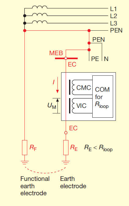
3.5 Stakeless methods (no probe, no auxiliary earth electrode) using a clamp-on ohmmeter
This is a variation on the measurement method described in section 3.4. This technique differs from that shown in figure 7 in that instead of inserting an earth resistance meter into the earthing conductor, a clamp-on ohmmeter (COM) is placed around the earthing conductor (see figure 9). The clamp-on ohmmeter contains both a current-to-voltage transformer (a voltage inducing clamp, VIC) and a current transformer (a current measuring clamp CMC).
The meter displays the resistance calculated as the quotient of the voltage induced by the VIC in the earthing conductor and the resulting test current registered by the CMC. In this case the resistance is the loop resistance Rloop, or more precisely the loop impedance (see section 3.4.1).
Another solution (no separate diagram provided) involves clamping two split-core current transformers around the earthing conductor, one of which functions like the voltage-inducing clamp VIC while the other corresponds to the current measuring clamp CMC that measures the test current. The clamps are connected to a special earth resistance meter (Fluke Earth Ground Tester 1623 or 1625). Depending on which of the Fluke meters is used, either EI-1623 or EI-1625 ‘selective/stakeless clamp set’ is required. The advantage in both cases is that the earthing conductor does not need to be disconnected, making measurement safer and quicker. The problem discussed in section 3.4.2 can also arise in these cases.
If this method is used to make measurements on consumer installations, they must be designed with a TN earthing system. The method is suitable for measuring the resistance to earth of a pylon in an overhead power transmission line if the clamps can be fitted around the earthing conductor.
Figure 9 Method as in figure – but with a clamp-on ohmmeter rather than an earth resistance meter
EC earthing conductor; VIC voltage-inducing clamp; CMC current measuring clamp; COM clamp-on ohmmeter.
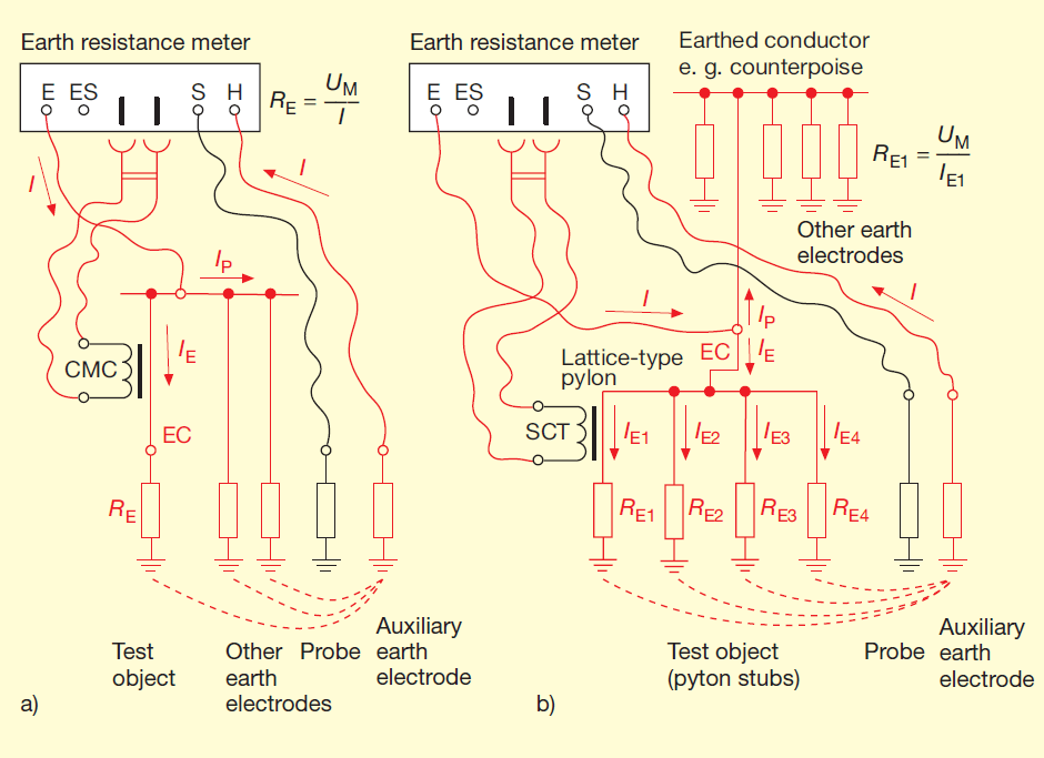
3.6 Selective earth resistance measurements using a probe, an auxiliary earth electrode and a clamp-on ohmmeter
The earth resistance measurement described in this section6) is used if the earth electrode under test cannot or should not be disconnected from other earth electrodes to which it is wired in parallel. This method is based on the technique using a probe and auxiliary earth electrode that is discussed in section 3.2, but in this variant (see figure 10a) a special earth resistance meter (Fluke 1623 or 1625) and an additional clamp-on current transformer (CMC) are required. The current measuring clamp CMC is clamped around the earthing conductor EC connected to the earth electrode under test and connected to a multi-pole socket on the earth resistance meter. When the meter is connected in this way and the rotary selector switch has been set appropriately, IP, the portion of the test current I flowing via the other parallel earth electrodes, has no effect on measurement result so that the branch current IE recorded by current measuring clamp CMC is solely responsible for determining the resistance to earth RE displayed by the meter.
Figure 10b) shows the measurement circuit used when dealing with a steel-lattice electricity pylon that cannot be electrically disconnected from the earthed conductor (e. g. counterpoise, PEN conductor or neutral conductor). As the pylon structure serves as the earthing conductor EC, it is clearly not possible to clamp a CMC around the earthing conductor as in figure 10a). In this case, measurements are made by consecutively clamping a splitcore transformer SCT (Fluke EI-162BN7)) around the four pylon legs that are connected to the four pylon stubs that act as earth electrodes. The earth resistance meter displays the resistances RE1 to RE4 consecutively. The resulting earth resistance RE of the four mast feet, which are connected to one another through the steel lattice structure, can be calculated by equation (5):
Figure 10 Selective earth resistance measurements using a probe, an auxiliary earth electrode and split-core current transformers
a) Test object whose earthing conductor can be clamped by a split-core current transformer;
b) Pylon whose legs can be clamped by a split-core current transformer near the foundation of the pylon IE part of test current flowing through the earth electrode under test to the auxiliary earth electrode; IE1 to IE4 parts of IE flowing in the pylon legs and stubs; IP portion of the test current flowing to the auxiliary earth electrode via the other parallel earth electrodes (current path through soil not shown in part b) of figure).
4) Induced voltage: approx. 60 mV; frequency: 2403 Hz; inner diameter of clamp jaw: 32 mm. Data provided without warranty. 5) Induced voltage: approx. 30 mV; frequency: 1667 Hz; inner diameter of clamp jaw: 23 mm. Data provided without warranty. 6) On its own, the expression ‘selective earth measurement’ is ambiguous, as other earth resistance measurement techniques are also selective, e.g. those presented in sections 3.4, 3.5 and 4.6.
4Measurement Methods That Draw Current From Supply
4.1 Measuring equipment
The meters used for this type of measurement are designed primarily for testing electrical safety systems that make use of residual current devices. To ensure the simplest and safest connection to the power supply, the meters are typically equipped with a flexible power cable and an earthed safety plug. The meters also have a socket S for the probe (see figures 11 and 13). The socket E is used to connect the meter to the earth electrode under test unless one of the cores (protective earth core) of the flexible power cable and the earth contacts on the plug are used for this purpose. As the test meters are classified as Class II equipment (see ref. [4], sec. 4.5), the core and the plug’s earth contact do not serve as protection against shock hazards.
The meters do not have their own power source unless this is needed for some other type of measurement. Some meters may have an additional connector socket for a current measuring clamp.
7) The jaws of the split-core transformer are dimensioned for large rectangular-section conductors such as the legs of high-voltage pylon
Figures 11 to 14 show the basic principles of the complicated circuitry inside these meters. In most of these meters, the actual measurement process (including any gradual increase in the test current that may be involved) is carried out automatically. Rather than displaying the measured voltage and current separately, the resistance to earth is computed and displayed digitally on the meter.
A selector switch enables the type of measurement, measurement technique, measurement circuit, parameter range and/or measurement sequence to be chosen. Most meters are fitted with a ‘START’ button to initiate the measurement process. User-friendly devices offer additional functions such as:
Multiple measurements with display of average result
Smoothing function
Display hold function
Data storage for transmitting or printing measurement results.
To provide protection against electric shock, the meter must switch off automatically as soon as it causes a fault voltage greater than 50 V in the earthing system being measured. If a variable resistor is used to increase the test current, the current must not exceed 3.5 mA at the beginning of the measurement (see ref. [6], sec. 4.7). Measurements in which the test current is increased gradually and measurements in which the current is only allowed to flow at maximum strength for a short period are both common.
The difficulty associated with drawing current directly from the power supply is that the measurement is made at the supply frequency and interference currents that originate in the power supply or that are carried via earth can easily introduce measurement errors. The larger the test current, the less effect these sources of interference will have. It is therefore expedient to work with a large test current. However, a large test current can itself be problematic when the meter is connected behind a residual current device, as it can cause the RCD to trigger. This can be avoided by using one of the following procedures:
Ensuring that the magnitude of the test current is only half that of the rated residual current IΔN of the RCD.
Connecting the meter in front of the RCD or to a circuit that is not equipped with an RCD.
According to the manufacturer Chauvin Arnoux the patented ‘ALT system’ used in its C.A 6115 N and C.A 6456 Earth Clamps enables these devices to make earth resistance measurements using a larger test current even if connected behind a 30 mA RCD.
Whenever interference effects may play a role, several measurements should be conducted and the results compared with one another.
Figure 11 Current-voltage methods that draw current directly from the power supply and that use a probe
a) Installation with TN system;
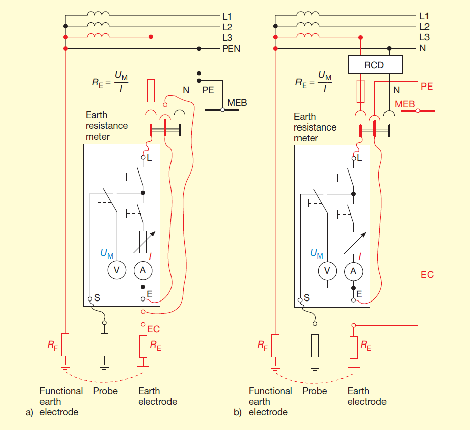
b) Installation with TT system EC earthing conductor; RCD residual current device; I test current; MEB Main earthing busbar; RF resistance of functional earth; RE earth resistance being measured; UM test voltage
Figure 12 Current-voltage methods that draw current directly from the power supply and that use the PEN or neutral conductor instead of a probe
a) Installation with TN system;
b) Installation with TT system
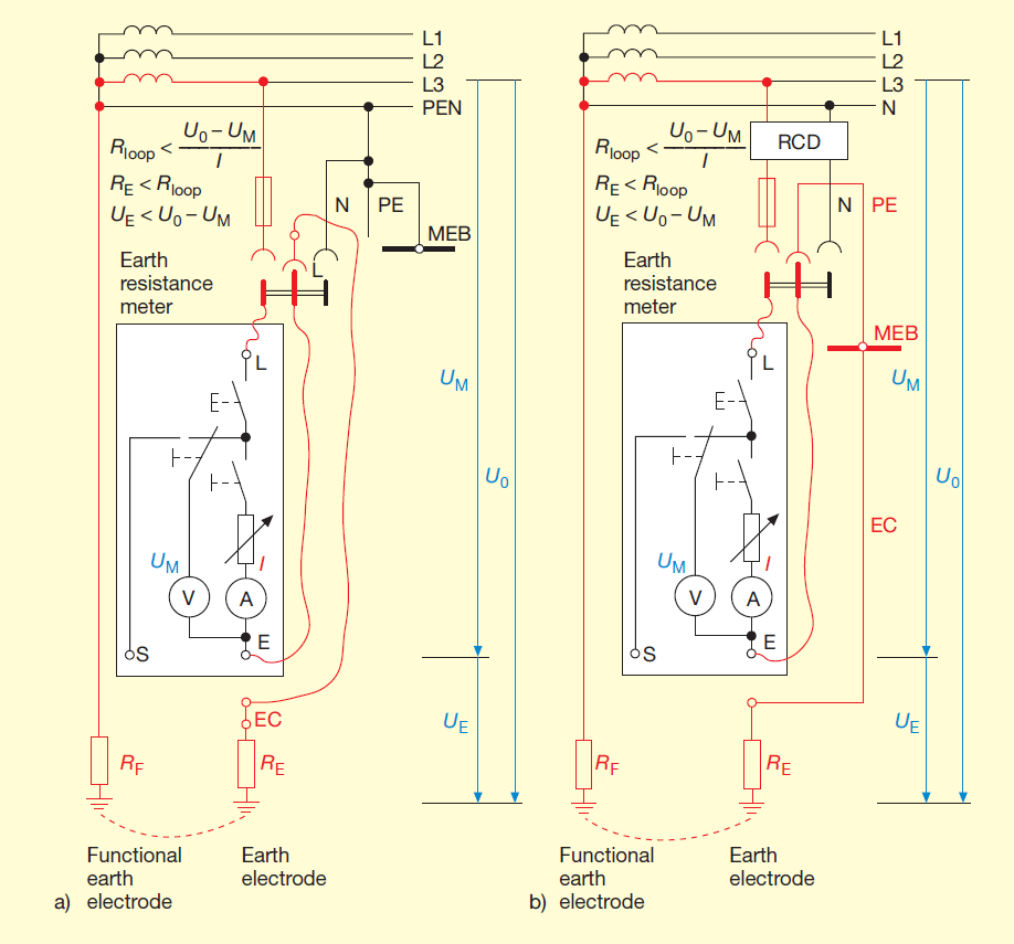
Figure 13 Current-voltage methods that draw current directly from the power supply and that do not use a probe
a) Installation with TN system;
b) Installation with TT system Rloop loop resistance; U0 conductor-to-earth voltage; UE voltage across tested earth electrode
Figure 14 Selective earth resistance measurement methods that draw current directly from the power supply and that use a probe and a clamp-on ammeter
a) Installation with TN system;
b) Installation with TT system IE portion of test current flowing to the earth electrode under test; IF portion of test current flowing to the other earth electrodes; CMC current measuring clamp
4.2 Connections to power supply and earth electrode
The meter is typically connected to the power supply via its earthed safety plug. If the plug is inserted incorrectly, no hazard arises but no measurement is possible. Although not shown in the figures, the internal circuitry of most of the meters only functions if the meter is connected to the phase conductor and to the neutral conductor.
The test current can induce accidental triggering of an upstream RCD. This may need to be taken into account when connecting the meter (see discussion in section 4.1 above). Depending on the type of meter used, the earth electrode to be measured is
either connected directly to socket E of the meter (see fig. 4 in section 2)
or (in most cases) is connected to the meter via the plug’s earth contact as shown in figures 11 to 14.
Connections between the earth electrode under test and other earth electrodes would yield erroneous results. It is for this reason that when measurements are made on consumer installations with a TN earthing system, the earthing conductor EC has to be separated from the main earthing busbar MEB (see figures 11a) to 14a)) as the latter is connected via the PEN conductor of the service cable and the supply network to other earth electrodes. Disconnection is not required in a TT system as the main earthing busbar is not linked to the neutral line of the supply network and the connection can be made as shown in figures 11b) to 14b).
4.3 Methods using a probe
This method is the most accurate of the techniques that draw current directly from the supply provided that the probe can be inserted into the soil at a suitable location. A schematic of the measurement set-up is shown in figure 11. The probe has to be located so that it is outside the sphere of influence of the earth electrode. The voltage UM between the sockets E and S generates the test current I in the earth electrode.
4.4 Method using the PEN conductor or neutral conductor instead of a probe
This measuring techniques can be used whenever it is not possible to insert a probe into the ground at the right location. In this method (see figure 12 ) the probe is replaced by connecting socket S of the meter to the PEN or PE conductor in a TN system or to the neutral conductor in a TT system. Caution! The neutral conductor must be treated as if it is live, even though it is earthed.
The value displayed by the meter includes the resistance to earth of the functional earth electrode. This will overestimate the resistance of the earth electrode and thus yield a value that errs on the side of safety.
The voltages generated by operating currents and by fault currents in the functional earth or in the PEN conductor or neutral conductor of the power supply system can result in erroneous measurement results. The accuracy of this technique is therefore lower than that achievable using the method described in section 4.3.
4.5 Method without a probe
This method (illustrated schematically in figure 11) involves measuring the resistance of a conductor loop via an earth return path. In this method, the voltage across the test object (UE) is not measured directly. It is determined as the difference between the potential drop between the phase conductor and earth when the test resistance is switched off (U0) and that when the test current I is flowing (UM). The resistance value measured includes the resistances of the functional earth, the transformer and the phase conductor. This will result in an overestimation of the earth resistance and thus yield a value that errs on the side of safety.
This method is particularly attractive as it can be performed with a minimum of effort. But it suffers from the weakness that supply load fluctuations that happen to occur simultaneously while the measurement is being made will cause significant additional measurement errors. To limit these errors, it is therefore expedient to work with a large test current. It is also advisable to perform numerous measurements, to reject any extreme values recorded and to compute the mean value from the remaining measurement data.
4.6 Selective earth resistance measurements using a probe and a clamp-on ammeter
The method selective earth resistance measurement8) is used if, for the purposes of the measurement, the earth electrode under test cannot or should not be disconnected from other earth electrodes to which it is wired in parallel. It is based on the method using a probe discussed in section 4.3, but in this variant (see figure 14) a special earth resistance meter (Chauvin Arnoux C.A. 6115N or C.A. 6456) and an additional current measuring clamp CMC are required. The current measuring clamp is connected to a multipole socket on the meter and the clamp jaws are placed around the earthing conductor EC connected to the earth electrode under test.
If the meter is connected in this way and if the rotary selector switch set appropriately, IP, the portion of the measuring current I flowing via the other parallel earth electrodes, has no effect on measurement result so that the branch current IE recorded by the current measuring clamp CMC is solely responsible for determining the resistance to earth RE displayed by the meter.
8) On its own, the expression ‘selective earth measurement’ is ambiguous, as other earth resistance measurement techniques are also selective, e. g. those presented in sections 3.4, 3.5 and 3.6.
References
[1] IEC 60364-4-41:205 Erection of power installations with nominal voltages up to 1000 V – Part 4-41: Protection for safety – Protection against electric shock. [2] Hering, E.: Schutzerder des TT-Systems (engl.: Protective earthing in the TT system). Elektropraktiker, Berlin 59 (2005) 5, p. 370-373. [3] IEC 60364-6:2006-02 Low-voltage electrical installations – Part 6: Verification. [4] IEC 61557-1:2007 Equipment for testing, measuring or monitoring of protective measures – Part 1: General requirements. [5] IEC 61557-5:2007 Equipment for testing, measuring or monitoring of protective measures – Part 5: Resistance to earth. [6] IEC 61557-6:2007 Equipment for testing, measuring or monitoring of protective measures – Part 6: Effectiveness of residual current devices (RCD) in TT, TN and IT systems. [7] IEC 61557-10:2000 Equipment for testing, measuring or monitoring of protective measures – Part 10: Combined measuring equipment for testing, measuring or monitoring of protective measures. [8] Hering, E.: Probleme mit einem der Erdungsmeßverfahren beim TN-System (engl.: Problems with an earth resistance measurement technique in a TN system). Elektropraktiker, Berlin 53 (1999) 9, p. 820-822. [9] Hering, E.: Durchgangsprüfungen an Erdungsanlagen [Continuity testing in earthing systems]. Elektropraktiker, Berlin 59 (2005) 11, p. 888- 891 und in diesem Sonderdruck. [10]DIN EN 62305-3 (VDE 0185-305-3):2006-10: Protection against lightning – Part 3: Physical damage to structures and life hazard.
Published by H. Markiewicz and A. Klajn, November 2014
ECI Publication No. Cu0120
Document Issue Control Sheet
Document Title:
Application Note – Earthing Systems: Fundamentals of Calculation and Design
Publication No:
Cu0120
Issue:
03
Release:
June 2003
Author(s):
H. Markiewicz and A. Klajn
Reviewer(s):
D. Chapman, S. Fassbiner
Document History
Issue
Date
Purpose
1
June 2003
Initial publication
2
November 2011
Upgrade by David Chapman for adoption into the Good Practice Guide
3
November 2014
Review with minor adaptations
Disclaimer
While this publication has been prepared with care, European Copper Institute and other contributors provide no warranty with regards to the content and shall not be liable for any direct, incidental or consequential damages that may result from the use of the information or the data contained.
SUMMARY
This Application Note discusses the principles of earthing electrode design with particular emphasis on earth potential distribution of various electrode geometries.
The electrical properties of the ground and variations according to type and moisture content are discussed. The equation for calculation of the earthing resistance and potential distribution for an idealized hemispherical earth electrode is derived. The concepts of step and touch voltages are discussed and the effect of earthing electrode geometry shown.
The concepts developed here are the basis for the practical guidance given in the Application Note Earthing Systems: Basic Constructional Aspects.
INTRODUCTION
The concept of modern integrated earthing systems was introduced in the Application Note Integrated Earthing Systems. In an integrated earthing system, all of the different earthing functions – lightning and short circuit protection, safety and electromagnetic compatibility – are designed and implemented as one entity.
This Application Note is concerned only with the part of an integrated system that is buried in the ground, called the earth or ground electrode, and covers fundamental aspects of design and calculation. A further Application Note, Earthing systems: Basic Constructional Aspects gives practical guidance on the design of ground electrodes and the calculation of their properties.
The earthing system is an essential part of power networks at both high- and low-voltage levels. A good earthing system is required for:
Protection of buildings and installations against lightning
Safety of human and animal life by limiting touch and step voltages to safe values
Electromagnetic compatibility (EMC) i.e. limitation of electromagnetic disturbances
Correct operation of the electricity supply network and to ensure good power quality
In modern practice these functions are provided by a single system designed to fulfill the requirements of all of them. Although some elements of an earthing system may be provided to fulfill a specific purpose, they are nevertheless part of one single system – standards require that all earthing measures within an installation are bonded together, forming one system.
BASIC DEFINITIONS [1, 2]
Earthing or earthing system is the total of all means and measures by which part of an electrical circuit, accessible conductive parts of electrical equipment (exposed conductive parts) or conductive parts in the vicinity of an electrical installation (extraneous conductive parts) are connected to earth.
Earth or ground electrode is a metal conductor, or a system of interconnected metal conductors, or other metal parts acting in the same manner, embedded in the ground and electrically connected to it, or embedded in the concrete, which is in contact with the earth over a large area (e.g. foundation of a building).
Earthing conductor is a conductor which connects a part of an electrical installation, exposed conductive parts or extraneous conductive parts to an earth electrode or which interconnects earth electrodes. The earthing conductor is laid above the soil or, if it is buried in the soil, is insulated from it.
Reference earth is that part of the ground, particularly on the earth surface, located outside the sphere of influence of the considered earth electrode, i.e. between two random points at which there is no perceptible voltages resulting from the earthing current flow through this electrode. The potential of reference earth is always assumed to be zero.
Earthing voltage (earthing potential), VE, is the voltage occurring between the earthing system and reference earth at a given value of the earth current flowing through this earthing system.
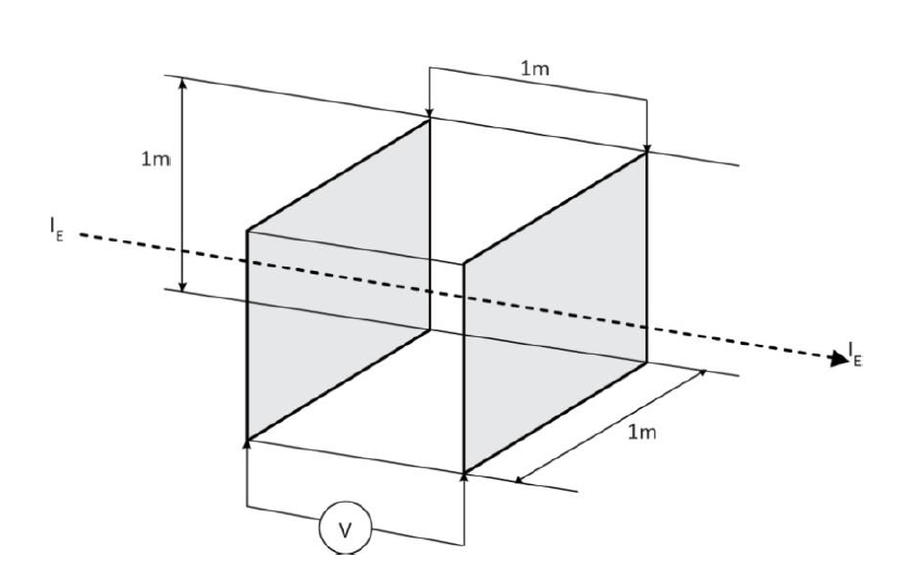
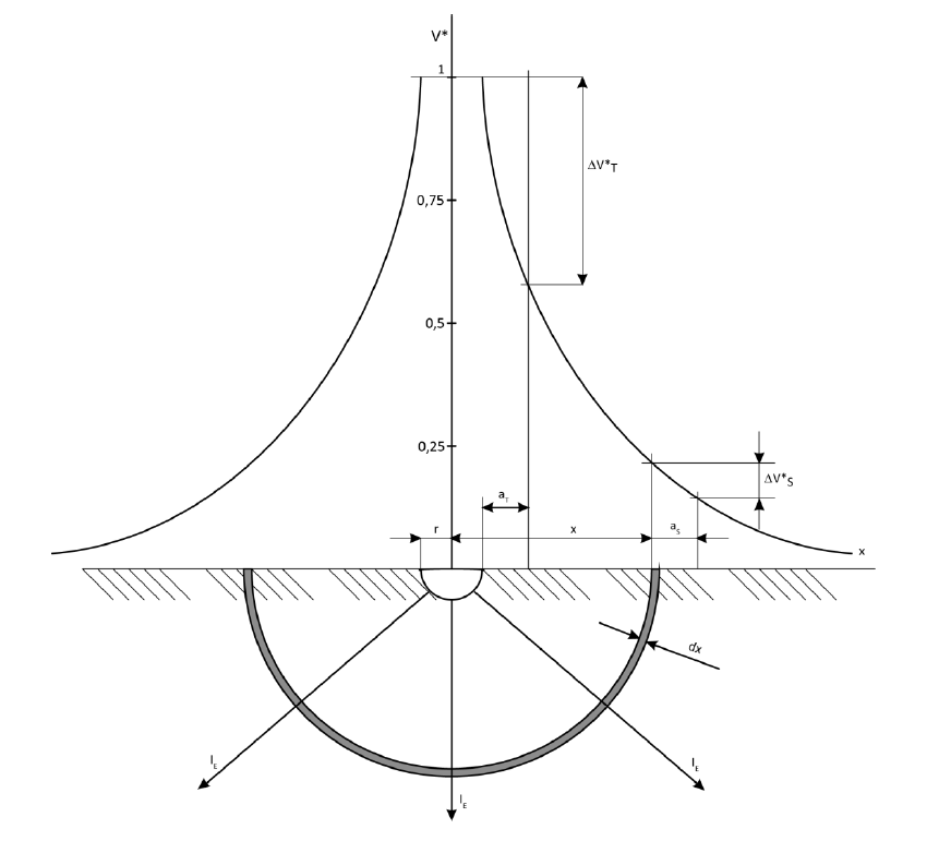
Earth resistivity ρ (specific earth resistance) is the resistance, measured between two opposite faces, of a one-metre cube of earth (See Figure 1). The earth resistivity is expressed in Ωm.
Earth surface potential,Vx, is the voltage between a point x on the earth’s surface and reference earth.
Figure 1 – Diagram illustrating the physical sense of earth resistivity ρ.
ELECTRICAL PROPERTIES OF THE GROUND
The electrical properties of the ground are characterised by the earth resistivity ρ. In spite of the relatively simple definition of ρ given above, the determination of its value is often a complicated task for two main reasons:
The ground does not have a homogenous structure, but is formed of layers of different materials
The resistivity of a given type of ground varies widely and is very dependent on moisture content
The calculation of the earthing resistance requires a good knowledge of the soil properties, particularly of its resistivity ρ. Thus, the large variation in the value of ρ is a problem. In many practical situations, a homogenous ground structure will be assumed with an average value of ρ, which must be estimated on the basis of soil analysis or by measurement. There are established techniques for measuring earth resistivity. One important point is that the current distribution in the soil layers used during measurement should simulate that for the final installation. Consequently, measurements must always be interpreted carefully. Where no information is available about the value of ρ it is usually assumed ρ = 100 Ωm. However, as Table 1 indicates, the real value can be very different, so acceptance testing of the final installation, together with an assessment of likely variations due to weather conditions and over lifetime, must be undertaken
Table 1 – Ground resistivity ρ for various kinds of the soil and concrete [2, 4].
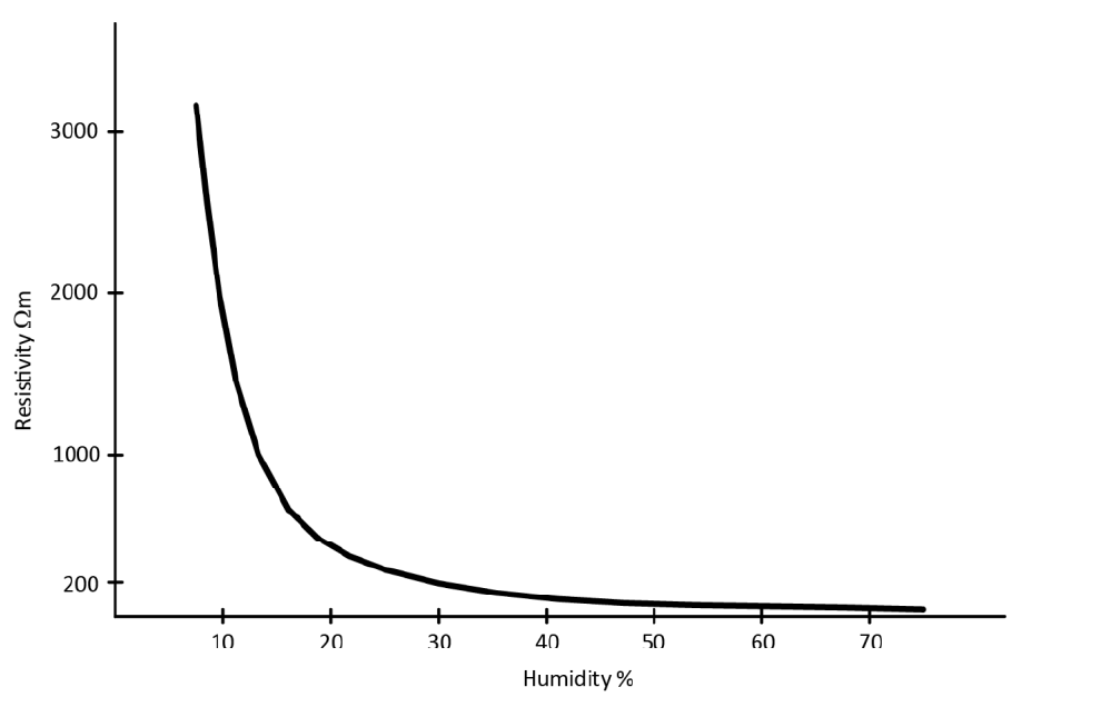
The other problem in determining soil resistivity is the moisture content, which can change over a wide range, depending on geographical location and weather conditions, from a low percentage for desert regions up to about 80 % for swampy regions. The earth resistivity depends significantly on this parameter. Figure 2 illustrates the relationship between resistivity and humidity for clay. One can see here that, for soil humidity values higher than 30 %, changes of ρ are very slow and not significant. However, when the ground is dry, i.e. values lower than 20 %, the resistivity increases very rapidly.
In regions with a temperate climate, for example in European countries, the earthing resistance changes according to the season of the year, due to dependence of soil humidity on earth resistivity. For Europe, this dependence has an approximate sine form, where the maximum value of earthing resistance occurs in February and the minimum value in August. The average value occurs in May and November. The amplitude in February is approximately 30 % larger than average, while in August it is about 30 % smaller than the average [4].
It must be remembered that the effect of freezing is similar to that of drying – the resistivity increases significantly.
For these reasons the calculations of earth resistance and the design of electrodes can only be performed up to a limited level of accuracy.
Figure 2 – Earth resistivity ρ of clay as function of soil humidity.
ELECTRICAL PROPERTIES OF THE EARTHING SYSTEM
The electrical properties of earthing depend essentially on two parameters:
Earthing resistance
Configuration of the earth electrode
Earthing resistance determines the relation between earth voltage VE and the earth current value. The configuration of the earth electrode determines the potential distribution on the earth surface, which occurs as a result of current flow in the earth. The potential distribution on the earth surface is an important consideration in assessing the degree of protection against electric shock because it determines the touch and step potentials. These questions are discussed briefly below. The earthing resistance has two components:
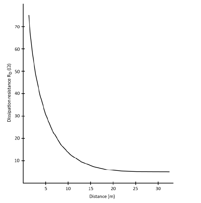
Dissipation resistance RD, which is the resistance of the earth between the earth electrode and the reference earth.
Resistance RL of the metal parts of the earth electrode and of the earthing conductor.
The resistance RL is usually much smaller than the dissipation resistance RD. Thus, usually the earthing resistance is estimated to be equal to the dissipation resistance RD. In the literature, ‘earthing resistance’ usually refers to the dissipation resistance.
Any earth connection made available by the supplier appears in parallel with the locally provided earth and may well be expected to have lower impedance at fundamental and harmonic frequencies than the local earth. However, the availability and characteristics of this path are beyond the designer’s control and hence should not be considered in the design of the earthing system which should be adequate for the required purpose in its own right.
EARTHING RESISTANCE AND POTENTIAL DISTRIBUTION
In AC circuits one must consider essentially the impedance of an earthing ZE, which is the impedance between the earthing system and the reference earth at a given operating frequency. The reactance of the earthing system is the reactance of the earthing conductor and of metal parts of the earth electrode. At low frequencies – the supply frequency and associated harmonics – reactance is usually negligible in comparison to earthing resistance, but must be taken into account for high frequencies such as lightning transients. Thus, for low frequencies, it is assumed that the earthing impedance ZE is equal the dissipation resistance RD, which is in turn assumed to be approximately equal to the earthing resistance, R:
The earthing resistance R of an earth electrode depends on the earth resistivity ρ as well as the electrode geometry. In order to achieve low values of R the current density flowing from the electrode metal to the earth should be low, i.e. the volume of earth through which the current flows should be as large as possible. Once the current flows from metal to earth it spreads out, reducing current density. If the electrode is physically small, e.g., a point, this effect is large, but is very much reduced for a plate where spreading is only effective at the edges. This means that rod, pipe, or wire electrodes have a much lower dissipation resistance than, for example, a plate electrode with the same surface area. Moreover, it is well documented in the literature that dc- and ac-induced corrosion increases with current density. Low current density extends electrode life.
The calculation of earthing resistance is usually performed under the assumptions that the ground is boundless and of uniform structure with a given value of resistivity. It is possible to determine exact equations for earthing resistance but, in practice, their usefulness is very limited, especially in case of complex and meshed earth electrodes where the mathematical relations become very complicated. Furthermore, even a small inaccuracy in value of the resistivity has a significant influence on the actual earthing resistance of meshed earth electrodes and it is often very difficult to determine the earth resistivity with the accuracy required. Because of this, exact theoretical equations of earthing resistance are usually used only for simple structures of earth electrodes in order to illustrate the relationship between the earth voltage, earth potential distribution and the earth current. For extended and meshed earth electrodes, approximations of earth resistance are used.
A basic model of the earth electrode configuration, used for illustrating the fundamental electrical properties, is a hemisphere embedded in the ground surface (Figure 3).
Figure 3 – Illustration of a notional hemispherical earth electrode, showing parameters required to calculate the earthing resistance and potential distribution on the ground surface (with ρ = const):
r – electrode radius
x – destination from the centre of the electrode
aT, aS – touch and step distances respectively
V* – relative value of the potential distribution
ΔV*T, ΔV*S – touch and step voltages respectively
The earth current flowing to such an electrode is assumed to flow radially to the earth. The surface of the hemisphere, as well as all hemisphere cross sections, dx, of the ground, are assumed to be equipotential, and the current lines are therefore perpendicular to these surfaces. Under these conditions the resistance of the hemisphere-ground-sheath of thickness dx and the radius x is expressed as follows (with ρ assumed constant):
The resistance of the hemisphere-earth electrode is given by:
The earth resistance depends significantly on how deep the electrode is sunk in the ground. This is because the moisture content is higher and more stable for deeper ground layers than for shallow layers. Layers near the surface are influenced more by seasonal and short-term weather variations and are subject to freezing. This problem is illustrated in Figure 4, for a vertical rod earth electrode, where one can see the considerable reduction of earthing resistance as the depth of penetration of a rod electrode increases. However, it is not always possible to place electrodes at the preferred depth for geological reasons, for example, where there are rocks or obstructions close to the surface or where the electrode system covers a large area.
Figure 4 – Example of dissipation resistance of a vertical rod earth electrode as a function of the depth d.
One can distinguish the following types of earth electrodes:
Simple surface earth electrodes in the form of horizontally placed strip or wire either as a single ended strip or a ring
Meshed electrodes, constructed as a grid placed horizontally at shallow depth
Cable with exposed metal sheath or armour which behaves similarly to a strip-type earth electrode
Foundation earth electrodes formed from conductive structural parts embedded in concrete foundation providing a large area contact with the earth
Rod electrodes which can consist of a pipe, rod, etcetera, and are driven or buried to a depth greater than 1 m and usually from 3 m to 30 m or more
The first four arrangements are surface earth electrodes, which usually consist of strip wire or band arranged as radial, ring or meshed electrodes, or a combination of these embedded at shallow depths of up to about 1 m. An important advantage of these constructions is the favourable surface potential distribution. Rod electrodes belong to so called deep earth electrodes, the advantage of these is that they pass through soil layers of different conductivity and are particularly useful in places where the shallow layers have poor conductivity. In this way it is easy to obtain an expected electrode resistance (Figure 4). Another advantage of rod electrodes is that they can be installed in places where there is a limited surface area available to install the electrode. However, surface potential distribution of rod electrodes is unfavourable, so in practice a combination of rod and surface earth electrodes are also used, in order to obtain both a good resistance and desirable surface potential distribution. Surface potential distribution is subject of the next section.
More detailed descriptions and basic equations concerning earth resistance of typical earth electrodes mentioned are given in the Application Note Earthing systems – Basic Constructional Aspects.
EARTHING VOLTAGE AND EARTH SURFACE POTENTIAL DISTRIBUTION
The earthing voltage and the distribution of the earth surface potential, arising from fault current flowing in the earthing system, are important parameters for protection against electric shock. The basic relations are shown on the earth model presented in the Figure 3.
The potential of any point located at distance x from the middle of earth electrode, in which earth current IE flows, can be formulated with the following equation:
and its relative value:
where VE is the earthing voltage, which is equal to the earthing potential (assuming that the potential of the reference earth is equal to zero). The earthing potential can be described as follows:
The potential difference between two points on the earth surface: one at distance x and other at distance x + aS, where aS is assumed to be equal to 1 metre, illustrates the step potential ΔVS, i.e. earth surface potential existing between two feet, when a person stands at that position on the earth surface:
and its relative value
where x ≥ r.
A similar relationship can be described for any other distances x and a. Particularly for x = r and a = aT = 1 m, formula (6) enables the calculation of the touch voltage, i.e. the voltage between a palm and a foot of a person who is just touching the earth electrode or metal parts connected to it:
and its relative value:
A practical illustration of touch and step voltages is shown in Figure 5. Persons A and B are subject to the touch potential while person C is subject to the step potential. The touch voltage VT is sometimes in the literature differentiated from the shocking touch voltage VTS (and step voltage VS from the shocking step voltage VSS).Voltages VT and VS are the pure values resulting from the potential distribution, whereas VTS and VSS consider the small changes in potential distribution caused by flowing of shocking current – i.e. including the distorting effect of the current flow through the person. In practice the difference between VS and VSS or VT and VTS is usually small, so that the same values for the respective potentials are assumed: VS≈ VSS and VT ≈ VTS
Figure 5 – Comparison of earth surface potential distribution during the current flow in the earthing system, for two earth electrode constructions:
(1) a rod electrode LHS
(2) a meshed electrode RHS
VE – earthing voltage
VT, VTS – touch voltage and shocking touch voltage respectively VS,
VSS – step voltage and shocking step voltage respectively
IT – shocking touch current
IK – short circuit current equal the current flowing to the earthing system
A, B, C – persons at various earth surface potentials
The left-hand side of Figure 5 shows the situation for a rod electrode while the right-hand side shows that for a meshed electrode. The rod electrode (1) has a low resistance but most unfavourable potential distribution while the meshed electrode (2) has a much flatter earth potential profile. The touch potential (person A) is considerably larger for the rod electrode (1) than for the meshed one (2), (person B). Step potentials (person C) are also less dangerous in case of the meshed electrode.
When a meshed earth is not possible, a ring electrode (as is common practice in Belgium and Germany, for example) provides an intermediate solution combining reasonable cost with reasonable safety.
The earthing resistance determines the value of earthing voltage, whereas the configuration of the earth electrode has significant influence on the potential distribution on the earth surface. Naturally, the configuration also influences the earthing resistance – a meshed electrode contacts a larger volume of earth – so both resistance and configuration need to be considered together. Note that, because meshed electrode systems cover large areas it is not practical to bury them deeply, so they are more susceptible to changes in soil moisture content. Improved stability of resistance can be achieved by including a number of long vertical rods in the mesh.
Figure 6 – The phenomenon of potential carryover. Earth surface potential distribution for two meshed earth electrodes;
a) meshed plane electrode,
b) plan of electrode;
c) electrode with two last elements placed deeper.
Meshed electrodes increase the surface area that experiences a voltage rise as the result of current flow to the earth electrode. Over the area of the mesh, equipotentiality exists, but at the periphery of the electrode there is a potential gradient as shown in Figure 6a. Although there is no touch potential – because the mesh extends beyond any metal structure by more than a meter – dangerous step voltages can occur. This situation can arise, for example, in the earthing system of a substation. In order to avoid this, the outer elements of the meshed earth electrode should be placed at a greater depth than the rest of the grid (Figure 6c).
PROPERTIES OF EARTHING AT HIGH IMPULSE CURRENTS
So far, the characteristics of earthing systems have been discussed assuming moderate current flow under steady-state conditions at the network frequency. Differences between steady-state and pulsed properties of an earthing system are caused mainly by:
Flow of currents with very high values, up to a few hundreds of kA
Very fast current rise times – typical lightning strikes reach a few hundred kA/µs [5]
Extremely high current density in the soil increases the electric field strength up to values which cause electrical discharges in small gaseous voids, decreasing the ground resistivity and earthing resistance. This phenomenon occurs mainly near the earth electrode, where the current density is highest, and the influence is most significant. The intensity of this phenomenon is especially high when the soil is dry or of high resistivity.
The inductance of metal parts of earth electrodes, which can be estimated as equal 1 µH/m, is usually neglected when considering earth impedance at the network frequency. However, inductance becomes an important parameter when the current slew rate is high, in the region of hundreds of kA/µs or more. During lightning strikes the inductive voltage drop (L di/dt) reaches very high values. As a result, remote parts of the earth electrode play a reduced role in conducting current to earth.
The earth resistance for pulse currents increases in comparison with its resistance for static conditions. Thus, increasing the length of earth electrodes over the, so called, critical length (Figure 7) does not cause any reduction of the earth impedance to transients.
Figure 7 – Maximal length lmax of lightning earth electrodes as a function of earth resistivity ρ.
During a lightning strike both the phenomena described above have an effect, but operate in opposite directions. The high earth current decreases resistance while the high frequency increases the impedance. The overall impedance can be higher or lower depending on which effect is dominant.
CONCLUSIONS
Earthing resistance and earth surface potential distribution are the main parameters characterising the electrical properties of the earthing system.
Electrical parameters of the earthing system depend on both soil properties and earth electrode geometry. Soil properties are characterised by earth resistivity, which changes over a wide range from a few Ωm up to few thousand Ωm, depending on the type of ground and its structure, as well as its humidity. As a result, it is difficult to calculate an exact value of earthing resistance. All relationships describing earthing resistance are derived with the assumption that the ground has a homogenous structure and constant resistivity.
Ideally, the earth surface potential should be flat in the area around the earth electrode. This is important for protection against electric shock, and is characterised by touch and step voltages. Rod electrodes have the most unfavourable surface potential distribution, while meshed electrodes have a much flatter distribution.
The behaviour of the earthing system for high transient currents should be considered. Very high current values diminish earthing resistance due to the strong electric field between the earth electrode and the soil, while fast current changes increase earthing impedance due to earth electrode inductance. The earthing impedance is, in this case, a superposition of both these events.
REFERENCES
[1] IEC 61936-1 “Power installations exceeding 1 kV a.c.”, 2011-11. [2] ABB Switchgear Manual, 10th edition, Düsseldorf, Cornelsen Verlag 1999. [3] IEC 60364-5-54:2011 “Electrical installations of buildings – Part 5: Selection and erection of electrical equipment – Chapter 54: Earthing arrangements and protective conductors” [4] Rudolph W., Winter O. EMV nach VDE 0100. VDE-Schriftenreihe 66. VDE-Verlag GmbH. Berlin, Offenbach, 1995. [5] IEC 62305:2010
Application Note – Earthing Systems: Fundamentals of Calculation and Design , H. Markiewicz and A. Klajn, November 2014, ECI Publication No Cu0120, Available from www.leonardo-energy.org
Ponemon Institute and Emerson Network Power are pleased to present the results of the 2013 Cost of Data Center Outages. First conducted in 2010, the purpose of this benchmark study is to determine the full economic cost of unplanned data center outages and is the second study in a two-part research series on the topic of data center outages.
The first study, 2013 Study on Data Center Outages, was released in September 2013 and was conducted to determine the frequency and root causes of unplanned data center outages. We believe both studies are important because of evidence that IT leaders are underestimating the economic impact unplanned outages have on their operations.
The 2013 Cost of Data Center Outages is the only benchmark study that attempts to estimate the full costs associated with an unplanned data center outage. According to the study, the cost of a data center outage has increased since 2010. The cost per square foot of data center outages now ranges from $45 to $95. Or, a minimum cost of $74,223 to a maximum of $1,734,433 per organization in our study. The overall average cost is $627,418 per incident. This benchmark analysis focuses on representative samples of organizations in the U.S. that experienced at least one complete or partial unplanned data center outage during the past 12months. The analysis was based on 67 independent data centers located in the United States.
Following are the functional leaders within each organization who participated in the study:
Facility manager
Chief information officer
Data center management
Chief information security officer
IT compliance leader
Utilizing activity-based costing, our methods capture information about both direct and indirect costs, including but not limited to the following areas:
Damage to mission critical data
Impact of downtime on organizational productivity
Damages to equipment and other assets
Cost to detect and remediate systems and core business processes
Legal and regulatory impact, including litigation defense cost
Lost confidence and trust among key stakeholders
Diminishment of marketplace brand and reputation
Following are some of the key findings of our benchmark research involving 67 data centers located throughout the nation.
Total cost of partial and complete outages can be a significant expense for organizations.
Total cost of outages is systematically related to the duration of the outage.
Total cost of outages is systematically related to the size of the data center.
Certain causes of the outage are more expensive than others. Specifically, IT equipment failure is the most expensive root cause. Accidental/human error is least expensive.
Part 2. Cost Framework
Utilizing activity-based costing, our study addresses nine core process-related activities that drive a range of expenditures associated with a company’s response to a data outage. The activities and cost centers used in our analysis are defined as follows:
Detection cost: Activities associated with the initial discovery and subsequent investigation of the partial or complete outage incident.
Containment cost: Activities and associated costs that enable a company to reasonably prevent an outage from spreading, worsening or causing greater disruption.
Recovery cost: Activities and associated costs that relate to bringing the organization’s networks and core systems back to a state of readiness.
Ex-post response cost: All after-the-fact incidental costs associated with business disruption and recovery.
Equipment cost: The cost of equipment new purchases and repairs, including refurbishment.
IT productivity loss: The lost time and related expenses associated with IT personnel downtime.
User productivity loss: The lost time and related expenses associated with end-user downtime.
Third-party cost: The cost of contractors, consultants, auditors and other specialists engaged to help resolve unplanned outages.
In addition to the above process-related activities, most companies experience opportunity costs associated with the data outage, which results in lost revenue, business disruption and average contribution. Accordingly, our cost framework includes the following categories:
Lost revenues: The total revenue loss from customers and potential customers because of their inability to access core systems during the outage period.
Business disruption (consequences): The total economic loss of the outage including reputational damages, customer churn and lost business opportunities.
Figure 1 presents the activity-based costing framework used in this research, which consists of 10 discernible categories. As shown, the four internal activities or cost centers include detection, containment, recovery, and ex-post response. Each activity generates direct, indirect, and opportunity costs, respectively. The consequence of the unplanned data center outage includes equipment repair or replacement, IT productivity loss, end-user productivity loss, third parties (such as consultants), lost revenues and the overall disruption to core business processes. Taken together, we then infer the cost of an unplanned data center outage.
Figure 1: Activity-based cost account framework
Part 3. Benchmark Methods
Our benchmark instrument was designed to collect descriptive information from IT practitioners and managers of data center facilities about the costs incurred either directly or indirectly as a result of unplanned outages. The survey design relies upon a shadow costing method used in applied economic research. This method does not require subjects to provide actual accounting results, but instead relies on broad estimates based on the experience of individuals within participating organizations.
The benchmark framework in Figure 1 presents the two separate cost streams used to measure the total cost of an unplanned outage for each participating organization. These two cost streams pertain to internal activities and the external consequences experienced by organizations during or after experiencing an incident. Our benchmark methodology contains questions designed to elicit the actual experiences and consequences of each incident. This cost study is unique in addressing the core systems and business process-related activities that drive a range of expenditures associated with a company’s incident management response.
Within each category, cost estimation is a two-stage process. First, the survey requires individuals to provide direct cost estimates for each cost category by checking a range variable. A range variable is used rather than a point estimate to preserve confidentiality (in order to ensure a higher response rate). Second, the survey requires participants to provide a second estimate for both indirect cost and opportunity cost, separately. These estimates are calculated based on the relative magnitude of these costs in comparison to a direct cost within a given category. Finally, we conduct a follow-up interview to obtain additional facts, including estimated revenue losses as a result of the outage.
The size and scope of survey items is limited to known cost categories that cut across different industry sectors. In our experience, a survey focusing on process yields a higher response rate and better quality of results. We also use a paper instrument, rather than an electronic survey, to provide greater assurances of confidentiality.
In total, the benchmark instrument contains descriptive costs for each one of the five cost activity centers. Within each cost activity center, the survey requires respondents to estimate the cost range to signify direct cost, indirect cost and opportunity cost, defined as follows:
Direct cost – the direct expense outlay to accomplish a given activity.
Indirect cost – the amount of time, effort and other organizational resources spent, but not as a direct cash outlay.
Opportunity cost – the cost resulting from lost business opportunities as a consequence of reputation diminishment after the outage.
To maintain complete confidentiality, the survey instrument does not capture company-specific information of any kind. Research materials do not contain tracking codes or other methods that could link responses to participating companies.
To keep the benchmark instrument to a manageable size, we carefully limited items to only those cost activities we consider crucial to the measurement of data center outage costs. Based on discussions with learned experts, the final set of items focus on a finite set of direct or indirect cost activities. After collecting benchmark information, each instrument is examined carefully for consistency and completeness. In this study, four companies were rejected because of incomplete, inconsistent, or blank responses.
The study was launched in July 2013 and fieldwork concluded in October 2013. The recruitment started with a personalized letter and a follow-up phone call to 563 US-based organizations for possible participation in our study.¹This resulted in 83 organizations agreeing to participate. Fifty organizations (67 separate data centers) permitted researchers to complete the benchmark analysis.
Three cases were removed for reliability concerns and two cases were removed because those data centers fell below the minimum size requirement. Utilizing activity-based costing methods, we captured cost estimates using a standardized instrument for direct and indirect cost categories. Specifically, labor (productivity) and overhead costs were allocated to four internal activity centers and these flow through to six cost consequence categories (see Figure 1).
Total costs were then allocated to only one (the most recent) data center outage experienced by each organization. We collected information over approximately the same time frame; hence, this limits our ability to gauge seasonal variation on the total cost of an unplanned data center outage.
¹The US-based companies contacted are all members of Ponemon Institute’s benchmark community. Most of these are organizations that have utilized the Institute’s benchmarking services for cost analysis over the past 12 years.
Part 4. Sample of Participating Companies & Data Centers
The following table summarizes the frequency of companies and separate data centers participating in the benchmark study. As reported, a total of 16 industries are represented in the sample.
Our final sample includes a total of 50 separate organizations representing 67 data centers – which is the unit of analysis. A total of five organizations were rejected from the final sample for incomplete responses to our survey instrument, thus resulting in a final sample of 67 data centers.
The following table summarizes participating data center size according to total square footage and the duration of both partial and complete unplanned outages. The average size of the data center in this study is 12,558 square feet and the average outage duration is 86 minutes.
Pie Chart 1 summarizes the sample of participating companies’ data centers according to 16 primary industry classifications. As can be seen, financial services and co-location services are the two largest industry segments representing 15 and 10 percent of the sample, respectively. Financial services companies include retail banking, insurance, brokerage, and investment management companies.
Pie Chart 1: Distribution of participating organizations by industry segment
Computed from 67 benchmarked data centers
Pie Chart 2 reports the percentage frequency of companies based on their geographic location according to six regions in the United States. The northeast represents the largest region (at 21 percent) and the smallest region is the Southwest (at 12 percent).
Pie Chart 2: Distribution of participating organizations by US geographic region
Computed from 67 benchmarked data centers
Part 5. Key Findings
Bar Chart 1 reports the cost structure on a percentage basis for all cost activities for FY 2010 and FY 2013. As shown, the cost mix has remained stable over the past three years. Indirect cost represents about half and opportunity loss represents 12 percent of total cost of outages.
Bar Chart 1: Percentage cost structure of unplanned data center outages
Table 3 summarizes the cost of unplanned outages for all 67 data centers. Please note that cost statistics are derived from the analysis of one unplanned outage incident.
Bar Chart 2 reveals significant variation across nine cost categories for FY 2010 and FY 2013. The cost associated with business disruption, which includes reputation damages and customer churn, represents the most expensive cost category. Least expensive involves the engagement of third parties such as consultants to aid in the resolution of the incident.
Bar Chart 2: Comparison of FY 2010 and FY 2013 activity cost categories
Bar Chart 3 provides the total cost of unplanned outages for 16 industry segments included in our benchmark sample. The analysis by industry is limited because of a small sample size; however, it is interesting to see wide variation across segments ranging from a high of almost $1 million (communications) to a low of almost $400,000 (hospitality).
Bar Chart 3: Distribution of total cost for 15 industry segments
Computed from 67 benchmarked data centers
Bar Chart 4 compares costs for partial unplanned outages and complete unplanned outages. Similar to 2010, complete outages are more than twice as expensive as partial outages.
Bar Chart 4: Cost for partial and total shutdown
Comparison of FY 2010 and FY 2013 results
Bar Chart 5 compares the average duration (minutes) of the event for partial and complete outages. In this year’s study, complete unplanned outages, on average, last 63 minutes longer than partial outages.
Bar Chart 5: Length in time (minutes) for partial and total shutdown
Comparison of FY 2010 and FY 2013 results
Graph 1 shows the relationship between outage cost and duration of the incident. The graph is organized in descending order by duration of the outage in minutes. Accordingly, observation 1 has the shortest duration and observation 57 has the longest duration. The regression line is derived from the analysis of all 67 data centers. Clearly, these results show that the cost of outage is linearly related to the duration of the outage.
Graph 1: Relationship between cost and duration of unplanned outages
Minutes of down time
Bar Chart 6 reports the minimum, median, mean and maximum cost per minute of unplanned outages computed from 67 data centers. This chart shows that the most expensive cost of an unplanned outage is over $16,000 per minute. On average, the cost of an unplanned outage per minute is likely to exceed almost $8,000 per incident.
Bar Chart 6: Total cost per minute of an unplanned outage
Comparison of FY 2010 and FY 2013
Graph 2 shows the relationship between data center size as measured by square footage and the total cost of unplanned outages. Observation 1 has the smallest and observation 59 has the largest data centers in square footage, respectively. The regression line is computed from the analysis of all 67 data centers. Similar to the duration analysis above, these results show that the cost of outage is linearly related to the size of the data center.
Graph 2: Relationship between cost and data center size (measured in square feet)
Bar Chart 7 reports the mean cost per square foot of unplanned outages based on all 67 data centers according to quartile. This chart shows that the most expensive cost of an unplanned outage is $95 per square foot for the smallest quartile of companies. The lowest average is $45 for larger organizations.
Bar Chart 7: Cost per square foot of data center
Quartile mean S.F. is bracketed value
Bar Chart 8 groups the sample of 67 data centers by the primary root cause of the unplanned outage. The “other” category refers to incidents where the root cause could not be determined. As shown, 24 percent of companies rate UPS system failure as the primary root cause of the incident. Twenty-two percent rate accidental or human error and 18 percent as a cyber attack as the primary root cause of the outage. IT equipment failure represents only four percent of all outages studied in this research.
Bar Chart 8: Root causes of unplanned outages
Comparison of FY 2010 and FY 2013 results
Bar Chart 9 reports the average cost of outage by primary root cause of the incident. As shown below, IT equipment failures result in the highest outage cost, followed by cyber crime. The least expensive root cause appears to be related to accidental/ human errors.
Bar Chart 9: Total cost by primary root causes of unplanned outages
Comparison of FY 2010 and FY 2013 results
$000 omitted
Part 6. Concluding Thoughts
The results of this year’s study clearly reflect shifting attitudes and trends since the original Study on Data Center Outages and Cost of Data Center Outages were released in 2010. The update to the Study on Data Center Outages, released in September 2013, indicated an increase of data center downtime awareness and an elevated sense of urgency surrounding availability, as well as a surge in cyber attacks related to availability. The companion Cost of Data Center Outages study, which analyzed 67 data centers across varying industry segments, indicates the significant increase in the cost of unplanned data center outages since 2010.
The 2010 studies fueled a global discussion on the consequences of data center outages at industry events such as AFCOM Data Center World and in dozens of IT and data center publications. It helped define and reinforce a business case for data center availability and safeguarding uptime, which was not previously a consideration for many business decisionmakers.
Recent high-profile outages also caught the attention of these business leaders. From the Superbowl to Twitter’s Fail Whale to outages of Amazon and Google, major disruptions to IT services around the globe helped bring downtime to the fore and reinforce not only the criticality of availability, but have also emphasized the dramatic financial cost associated with unplanned downtime.
With today’s data centers providing more critical, interdependent devices and IT systems than ever before, the 41 percent increase in cost from 2010 was remarkably higher than expected. The results underscore the importance of minimizing the risk of downtime that can potentially cost thousands of dollars per minute. The expectation that uptime is now a baseline assumption and there is an urgency to deliver it in order to save on costs, reverberates through the findings of the study.
Industries with revenue models dependent on the data center’s availability to deliver IT and networking services to customers – such as telecommunications service providers and ecommerce companies – and those that deal with a large amount of secure data – such as defense contractors and financial institutions – continue to incur the most significant costs associated with downtime. The highest cost of a single event was more than $1.7 million.
Those same industries did see a slight decrease (two-to-five percent) compared to 2010 costs, while those organizations that traditionally have been less dependent on their data centers saw a significant increase. The largest increase was in the hospitality sector, which saw a 129 percent increase; followed by the public sector (116 percent), transportation (108 percent) and media organizations (104 percent).
As there is an increasing need for a growing number of companies and organizations to adapt to a more social, mobile and cloud-based model, the criticality of minimizing the risk of downtime and committing the necessary investments is greater than ever before. This report should serve as a resource for those needing to make more informed business decisions regarding the cost associated with eliminating vulnerabilities and anticipating the costs associated with inaction.
Part 7. Caveats
This study utilizes a confidential and proprietary benchmark method that has been successfully deployed in earlier Ponemon Institute research. However, there are inherent limitations to benchmark research that need to be carefully considered before drawing conclusions from findings.
Non-statistical results: The purpose of this study is descriptive rather than normative inference. The current study draws upon a representative, non-statistical sample of data centers, all U.S.-based entities experiencing at least one unplanned outage over the past 12 months. Statistical inferences, margins of error and confidence intervals cannot be applied to these data given the nature of our sampling plan.
Non-response: The current findings are based on a small representative sample of completed case studies. An initial mailing of benchmark surveys was sent to a benchmark group of over 560 organizations, all believed to have experienced one or more outages over the past 12 months. Sixty-seven data centers provided usable benchmark surveys. Nonresponse bias was not tested so it is always possible companies that did not participate are substantially different in terms of the methods used to manage the detection, containment, and recovery process, as well as the underlying costs involved.
Sampling-frame bias: Because our sampling frame is judgmental, the quality of results is influenced by the degree to which the frame is representative of the population of companies and data centers being studied. It is our belief that the current sampling frame is biased toward companies with more mature data center operations.
Company-specific information: The benchmark information is sensitive and confidential. Thus, the current instrument does not capture company-identifying information. It also allows individuals to use categorical response variables to disclose demographic information about the company and industry category. Industry classification relies on self-reported results.
Unmeasured factors: To keep the survey concise and focused, we decided to omit other important variables from our analyses such as leading trends and organizational characteristics. The extent to which omitted variables might explain benchmark results cannot be estimated at this time.
Extrapolated cost results. The quality of survey research is based on the integrity of confidential responses received from benchmarked organizations. While certain checks and balances can be incorporated into the survey process, there is always the possibility that respondents did not provide truthful responses. In addition, the use of a cost estimation technique (termed shadow costing methods) rather than actual cost data could create significant bias in presented results.
Appendix 1: Summarized data for 67 benchmarked data centers
The following table summarizes the total cost of unplanned outages for 67 data centers. The activity cost column summarizes detection, containment, recovery, and ex-post response costs.
If you have questions or comments about this report, please contact us by letter, phone call or email:
Ponemon Institute LLC
Attn: Research Department, 2308 US 31 North, Traverse City, Michigan 49686 USA
Ponemon Institute is dedicated to independent research and education that advances responsible information and privacy management practices within business and government. Our mission is to conduct
high quality, empirical studies on critical issues affecting the management and security of sensitive information about people and organizations.
As a member of the Council of American Survey Research Organizations (CASRO), we uphold strict data confidentiality, privacy and ethical research standards. We do not collect any personally identifiable information from individuals (or company identifiable information in our business research). Furthermore, we have strict quality standards to ensure that subjects are not asked extraneous, irrelevant or improper questions.
This paper discusses the causes of Total Harmonic Distortion, how it is calculated, measured, and how it can impact a power distribution system.
Total Harmonic Distortion (THD) can be a challenging concept because of the complexity of the power system and its many individual components. THD is better understood when a power system is defined by its simplest parts– the power source and load, as shown in Figure 1.
Figure 1. Most basic parts of a power system
Because the load affects the current draw on a system, the power quality of the system is often affected as well, depending on the type of load. Loads can be either linear or non-linear. A linear load draws current that is sinusoidal in nature and has smooth current and voltage transitions, so generally this does not distort the waveform as seen in Figure 2.
Figure 2. Ideal sine wave with a linear load provided to the source
Many home appliances such as electric hot water heaters, base board heat, irons, and incandescent lighting have mostly resistive loads, which are relatively linear. Harmonic distortion is not usually caused by the power generation or distribution system itself and was not really an issue before 1960. Around this point in time changes in technology began to contribute to changes in customer load. Non-linear components such as diodes and SCR (or thyristors) started to be incorporated into household devices and appliances.
Some devices that have been known to present nonlinear loads to the power grid include AC/DC converters, motor speed controls / light dimmers, adjustable frequency drives, copiers, battery chargers, UPS, and also items such as electric welders, electronic ballast, and arc furnace. Higher energy efficiency lighting and government phasing out of incandescent light bulbs is driving consumers to replace old incandescent light bulbs with compact fluorescent lamps (CFL), light emitting diode (LED) and electron stimulated luminescence (ESL) type lighting. This type of lighting, while very energy efficient, does not provide a linear load such as incandescent light bulbs provide. In fact, the ESL beats out the energy efficiency of the CFL and LED hands down but has a power factor of 0.95 to 0.99 where the CFL and LED are in the 0.5 to 0.8 range. Another new source of harmonic distortion comes from variable motor speed controls currently being introduced in many high-efficient heat pumps. These non-linear devices present a non-linear load to the power source causing large distortions to the source waveform as shown in Figure 3.
Figure 3. Distorted waveform caused by non-linear loads
Non-linear loads cause waveform distortion, drastically changing the shape of a power source’s waveform. All sine waves are composed of harmonics which are multiples of the fundamental waveform. In the United States, the power line frequency is 60 Hz, so multiples of 60 Hz make up the sinusoidal power waveform. Harmonics can be defined as a steady state distortion of the fundamental frequency (e.g., 60 Hz for power lines). It is important to point out that a sine wave is made up of both even and odd harmonics. Non-linear loads usually cause odd-order harmonics to be more pronounced and problematic in a power distribution system. This is because most electrical loads, except for half-wave rectifiers, produce symmetrical current waveforms. This means that the positive half of the waveform is a mirror image of the negative half. This results in only odd harmonic values being present. A half-wave rectifier can produce even harmonics in addition to the odd ones. The illustration shown in Figure 4 demonstrates the relationship between the fundamental and the odd harmonics caused by nonlinear loads.
Figure 4. Relationship between the fundamental and odd order harmonics
Another factor that can sometimes cause an increase in harmonic problems are capacitor banks that are used to correct the power factor of inductive loads. If the capacitor resonance is at some multiple of the fundamental, it can actually magnify harmonic problems. Careful design and consideration is important when installing capacitor banks and it is also important to monitor THD and power factor because the inductive load may change from time to time as a result of new loads presented by customers.
The graph in Figure 5 shows the relationship of the fundamental frequency and some of the lower odd harmonics that add together to form the resultant.
Figure 5. The relationship of the fundamental frequency and lower odd harmonics that add together to form the resultant
THD
Total harmonic distortion in reference to (F) fundamental represents the ratio, in percent, of the voltage/current harmonic components relative to the voltage/current of the fundamental. When the reference is not indicated (i.e. simply THD), then it is usually assumed the reference is fundamental and not THD-R which is a different measurement. For power systems, THD or THD-F is a better measurement to use. Below is an equation used to calculate THD where Vn is equal to the Magnitude of the nth harmonic.
One of the main reasons to measure THD and accurately assess its value is so the operator can evaluate and monitor the system’s distortion level over time. This allows the operator to see what changes need to be made to the power system before the distortion levels elevate to a point where they could damage the system.
Some issues that high THD can cause are overheating transformers, issues with the proper operation of 3-phase motors, increase hysteresis losses, unacceptable neutral-to-ground losses, decreased kVA capacity, inaccurate power measurements, interference to communication systems such as telephone and radio, breaker tripping and fuse blowing, damage to capacitor banks, damage or interference to electronics, and the list goes on.
Technology and growth tend to progressively load the grid with more and more non-linear loads causing total THD to grow. It is very important to monitor the system to head off issues before they shut down the power system and result in damage to critical equipment. The increase in harmonic content may require some systems to be evaluated for proper transformer derating or upgrades to power distribution systems with K-rated transformers to reduce overheating or early life failures.
With ProVision and most PMI recorders, accurate measurement can be taken and displayed on many facets of power quality including Total Harmonic Distortion. The ProVision default for THD is F or fundamental but if desired by the operator, THD-R can easily be displayed by right-clicking on THD-F while in the Harmonic Analysis Magnitude Graph mode. If more detail is needed on the harmonics, press the F key while the cursor is on the graph. This removes the fundamental frequency allowing the graph to scale making the smaller, higher harmonics clearly visible. This could be very useful in areas where THD presents an issue to power quality such as a power related-issue with a 3 phase motor overheating, or communication interference. Figure 6 shows an example of a harmonic analysis report used to collect data on the LED lamp.
Figure 6. Example harmonic analysis report used to collect data from a Revolution on an LED lamp
Figure 7 shows a comparison of THD of a regular incandescent 60 Watt bulb, a CFL and a LED type light.
All PMI recorders with harmonic capability can record THD stripcharts, which gives a min, max, and average value for each interval period.
Incandescent 60 Watt bulb type light
CFL type light
LED type light
Figure 7. Data from a Revolution comparing THD o f a regular incandescent 60 Watt bulb, a CFL and a LED type light.
Figure 8 shows a mixed stripchart graph with voltage and current THD. The upper plot is channel 1 voltage THD, and the lower plot is channel 1 current THD. Looking at voltage and current THD together can help determine whether a monitored load is contributing to voltage THD, or just being affected by it. Figure 9 shows a Current THD Daily Profile. Like other daily profiles, the THD profile represents the average THD on a 15-minute basis throughout an “average” day, computed by averaging through the entire recording period. Here we see that the THD drops during the day, and rises during the night. This likely indicates more linear loads during the day, and as those turn off at night, the mix skews towards non-linear harmonic producing loads. Unlike the THD stripcharts, THD Daily Profiles are always enabled in a recorder with harmonic capability, so they can be useful if THD becomes a question after a recording is complete.
Figure 8. Mixed stripchart graph with voltage and current THD
Figure 9. Current THD daily profile
CONCLUSION
THD, simply put, is the measurement of the amplitudes of the harmonics that a nonlinear system introduces relative to the amplitude of the fundamental frequency. As new regulations are put into place to help conserve our natural resources by improving system efficiency, it is essential to have the proper monitoring systems in place to evaluate the power distribution system. Sometimes improvements in one area can cause problems in another area. Harmonics that are caused by nonlinear loads can cause issues such as transformer failures, excessive heating of motors, electronic device failures, and communication issues related to RFI and noise ingression into the communication system. With the right monitoring equipment and integrated software, and an understanding of power quality fundamentals, it is possible to continually and effectively assess overall system health and prevent potential system failure.
Published by Anthony (Tony) Hoevenaars, P. Eng , President and CEO Mirus International Inc.
INTRODUCTION
Active Front End (AFE) Drive manufacturers will claim that their technology provides the best solution for treatment of harmonics associated with variable frequency drives (VFDs). They are quick to point out benefits over standard 6-Pulse VFDs equipped with diode bridge rectifiers such as, reduced line current harmonics, improved power factor and inherent regenerative capabilities. But they will hide the fact that current harmonics are much higher when measured above the 50th and that very serious problems can result from the introduction of these higher frequency harmonics. Also, they will downplay a substantial loss in efficiency due to the increased losses in the input IGBTs.
The reality is:
AFE’s are not the best solution for a low harmonic VFD.
A properly designed Wide Spectrum Passive Filter, such as the Lineator AUHF, can outperform AFE especially when harmonics up to the 100th are taken into consideration.
AFE’s generate high frequency harmonics which can have more serious consequences than low frequency harmonics. As a passive device, Lineator AUHF cannot introduce high frequency harmonics and will, in fact, help reduce them when they are present.
If there is a mixture of 6-Pulse and AFE Drives on the same switchboard, the ripple in voltage from the AFE Drive can raise the DC bus voltage in the 6-Pulse VFDs creating overvoltage conditions.
Although an active solution, AFE’s still require input passive filters (LCL and EMI/RFI filters) to control switching frequency harmonics and to attenuate ripple in the mains side voltage and current.
LCL and EMI/RFI filters are more likely to resonate with the power system at rectifier harmonic frequencies (ie. 5th, 7th, 11th, etc.) than the Lineator AUHF. Also under lightly loaded conditions, the reactive power of the LCL capacitors can cause over-excitation of generators.
AFE’s generate significant levels of ground leakage current which can cause inadvertent ground fault trips and failure of sensitive equipment.
AFE losses are significantly higher and efficiencies much lower than a 6-Pulse VFD with Lineator AUHF.
AFE TOPOLOGY VS LINEATOR/6-PULSE VFD
Fig. 1a shows a typical AFE drive topology. The problems associated with the operation of AFE rectifiers are related to the converter design characteristics, switching frequency and interaction with the power system. You will note that ahead of the input bridge is a passive LCL filter. The function of this filter is to reduce the switching frequency harmonics introduced by the IGBTs. All AFE manufacturers, however, include LCL filters that are only minimally effective because a more effective filter would be much more expensive and physically larger. In fact, this passive filter would very likely be larger and more expensive than the Lineator AUHF that provides equivalent current harmonic mitigation on a simple 6-Pulse VFD (Fig 1b). Both topologies have an input passive filter but the Lineator/6-Pulse VFD topology is much simpler, more reliable and less expensive.
Fig. 1a: AFE Drive topology with LCL filter
Fig. 1b: 6-Pulse Drive topology with Lineator AUHF
AFE INTRODUCES HIGH FREQUENCY HARMONICS
In order to reduce input current harmonics, AFE Drives use IGBTs instead of a diode bridge rectifier. Current harmonics can be controlled through the switching action of the IGBTs but in so doing, switching frequency harmonics are introduced. Fig. 2 shows various measurements taken at a Paper Mill equipped with AFE Drives, by the authors of a paper on ‘Practical Problems Associated with the Operation of ASDs Based on Active Front End Converters in Power Distribution Systems’ [1]. They compare Ph-to-Gnd voltages and input currents while operating the AFE Drives as simple 6-Pulse Rectifiers and in full AFE operation.
Both operations show Ph-to-Gnd voltage with high frequency components but during AFE operation these distortions are substantially worse. Input current measurements show much lower levels of low frequency harmonics than in 6-Pulse operation but the high frequency ripple is very obvious in the waveform and the spectrum reflects this ripple with higher bars around the 50th.
With a band of harmonics near the 50th, the IGBTs on these Drives would be switching at around 2 – 3 kHz. With higher switching frequencies, the harmonic band would move out to higher harmonic orders. In many cases, these are well above the 50th where almost all power quality analyzers do not measure. Despite AFE Drive manufacturers’ efforts to ignore them, these higher frequency harmonics do certainly exist and most definitely can wreak havoc with connected equipment. These failures can be very difficult to diagnose even for trained power quality professionals.
Fig. 2: Variable Frequency Drive Voltage and Current Waveforms and Spectrums for an AFE Drive in a Paper Mill [1]
When AFE Drives are used on marine vessels with weak generator supplies, this problem can become even worse. The American Bureau of Shipping (ABS) has acknowledged this in several locations in Section 13 of its ‘Guidance Notes on Control of Harmonics in Electrical Power Systems’, such as:
iii) Total harmonic current distortion (Ithd), harmonic current spectrum up to 50th harmonic (or up to 100th for equipment with “active front ends”) and total magnitude of total harmonic current per unit, per circuit and per installation at rated load, as applicable. [2]
Fig. 3 shows frequency spectrums of the voltage at the Bridge Distribution Panel of a catamaran equipped with Main and Propulsion AFE Drives [3]. Measurements were taken over three frequency bands – up to 50th harmonic, 50th to 10 kHz and 10 kHz to 50 kHz. Although the voltage harmonics were very low in the lower frequency range (VTHD = 1.68%), they were very high in the frequency range above the 50th (VTHD = 8.14%) with a band around 3450 Hz (69th harmonic) produced by the AFE Drives operating at a 3.6 kHz switching frequency [3]. Most power quality analyzers that only measure up to the 50th harmonic would not have highlighted these high distortion levels.
These higher frequency harmonics will undoubtedly cause problems with connected equipment such as standard AC 6-Pulse VFDs, including those manufactured by the same supplier as the AFE Drives. The following statement is from the ‘Practical Problems’ paper sited earlier.
“From the power distribution point of view, the AFE rectifier operates as a current source, and as such injects high frequency current harmonics into the grid. If ASDs that use diode-based rectifiers (standard ASD) are connected to the same ac grid, the high frequency current components are pushed into their dc bus. This is due to the fact that they offer a low impedance path to these high frequency current components (due to the dc link capacitor presence), overloading the respective converter. Moreover, if the standard ASD is operating at light load, its dc bus voltage will tend to increase until the converter shuts down, hopefully by means of the dc link over voltage protection.” [1]
Fig 3: Voltage harmonic spectrum of a Marine Vessel with Main and Auxiliary Propulsion AFE Drives [3]
The authors of [1] also noted that the high speed IGBT switching action of AFE Drives introduces ground leakage currents (common-mode) that can cause inadvertent operation of ground fault protection equipment. Fig. 4 shows the neutral-to-ground voltage and currents of an AFE Drive running in both 6-Pulse operation and AFE operation. High frequency common-mode noise increases substantially while in AFE operation.
Fig. 4: Variable Frequency Drive Neutral-to-Ground Voltage and Current for an AFE Drive in a Paper Mill [1]
LINEATOR AUHF MATCHES AFE IN REDUCTION OF LOW FREQUENCY HARMONICS (UP TO 50th) WITHOUT INTRODUCING HIGH FREQUENCY HARMONICS
Lineator AUHF is a series connected, wide spectrum, passive harmonic filter designed to eliminate harmonics generated by 3-phase, 6-Pulse variable frequency drives. It performs as well as an Active Front End Drive in reducing harmonics in the low frequency range (up to 50th harmonics) while substantially outperforming AFE in the high frequency range. Lineator will provide some reduction in high frequency harmonics while the AFE Drive actually introduces these more damaging harmonics into the power system as described earlier.
The Lineator AUHF consists of a reactor with multiple windings on a common core and a relatively small capacitor bank (Fig. 5). This design exploits the mutual coupling between the windings to improve harmonic mitigation performance, making it far superior to conventional passive filter solutions. To prevent importation of upstream harmonics, the resonant frequency, as seen from the input terminals, is near the 4th harmonic, comfortably below the predominant harmonics of 3-phase rectifiers.
One key advantage of the unique reactor design is that it allows for the use of a significantly smaller capacitor bank (< 15% reactive power as a percent of the full load rating). This reduces voltage boost and reactive power at no load to ensure compatibility with generators. All other passive harmonic filter solutions introduce higher capacitive reactive power at light loads (typically 30% to 40%). Even the LCL filters on AFE Drives have higher capacitive reactance than the Lineator AUHF.
The filter is connected in series between the main supply and the drive. Current Total Harmonic Distortion (ITHD) is typically reduced to < 6% (a < 5% ITDD version is available) when applied to a 6-pulse AC PWM drive regardless of whether the drive is equipped with an AC or DC reactor or no reactor at all.
Lineators can be applied to AC drives with diode or SCR pre-charge input rectifiers ranging in size from 5HP/4kW to 3500HP/2600kW. They can be applied to single or multiple drives but only drive loads should be connected as the filter is designed specifically for rectifier operation. The filter can usually be retrofitted to existing drives without the requirement for drive modifications, whether for single drive or for multiple drive applications. A model is also available for operation on fully controlled SCR bridges, as used in DC Drives.
Figures 6 and 7 provide typical performance results measured in the Mirus Harmonics & Energy Lab on a Lineator AUHF. They show voltage and current waveforms and spectrums at the input to the Lineator measured up to the 500th harmonic using an ION 7650 Power Quality Analyzer.
Fig. 6: Input Current Waveform and Spectrum for 200HP, 480V Lineator AUHF
Fig. 7: Input Voltage Waveform and Spectrum for 200HP, 480V Lineator AUHF
Current Total Harmonic Distortion (ITHD) is only 5.12% even when all harmonics up to the 500th are included. Clearly noticeable is that, unlike the AFE Drive, there are extremely low levels of harmonic currents past the 50th.
Voltage Total Harmonic Distortion (VTHD), including all harmonics up to the 500th, is only 2.54%. This is well below the 5% maximum recommended by IEEE Std 519. Again, the harmonics above the 50th are virtually non existent, while for the AFE Drive, these were the highest harmonics present.
LINEATOR AUHF’s DESIGN PROTECTS AGAINST POWER SYSTEM RESONANCE
As a series connected passive filter, the Lineator’s combined inductance and capacitance presents a resonant frequency to the upstream power system. To prevent inadvertent resonance with the power system at a common characteristic harmonic frequency, the input resonant frequency is designed near the 4th harmonic to be comfortably below the 5th and other 6-Pulse rectifier harmonics.
Fig. 8a and 8b show a simple power system 1-Line and its equivalent diagram. Fig. 8c shows the reactance curves of the Lineator AUHF and the resonance point which occurs where these curves intersect. Since power systems are inherently inductive (unless installed Power Factor Correction capacitors are overcompensating which should always be avoided), the inductance curve will shift upwards moving the resonant frequency lower and further away from characteristic harmonics (Fig. 8d).
Fig 8: Lineator AUHF and Power System Resonance
The passive LCL and EMI/RFI filters required by AFE Drives, on the otherhand, are always tuned at a frequency above the 5th harmonic. The added inductive reactance of the power system will then lower the overall resonant frequency. When the resultant frequency matches a predominant harmonic on the power system, resonance will occur with its serious consequences. Therefore, the AFE Drive is much more susceptible to power system resonance than the Lineator AUHF.
AFE HAS HIGHER LOSSES RESULTING IN LOWER EFFICIENCY
Although the introduction of high frequency harmonics should in itself be enough justification to avoid the use of AFE Drives that do not have sufficient input passive filtering, there are many other reasons why the Lineator AUHF combined with a simple 6-Pulse VFD is a better solution. One significant reason is the higher losses and lower efficiency resulting from the operation of the input IGBT rectifier of the AFE.
Tables 1 and 2 show a major electrical manufacturer’s technical data for their AFE and 6-Pulse Drives, respectively. Table 3 provides a comparison of electrical losses and efficiency using the power loss statistics of a 75 kW (100 HP) and 400 kW (500 HP) Drive from these tables. With the losses of a Lineator AUHF added to the 6-Pulse VFD, this combination is still 1.7% more efficient than the AFE Drive. It is important to note that the stated AFE losses are for operation at the lowest IGBT switching frequencies. Losses increase with higher switching rates, further widening the efficiency gap.
Table 1: Technical Data for AFE Drives of a Major Drive Manufacturer [7]
Table 2: Technical Data for 6-Pulse VFDs of the same Drive Manufacturer [8][9]
Table 3: Efficiency Comparison – AFE vs 6-P VFD with Lineator
difference in efficiency can result in very substantial savings in energy and operating costs. The following example on a 400kW VFD calculates the annual savings when using the 6-P with Lineator vs an AFE Drive:
Therefore, by using a Lineator and 6-pulse VFD under the conditions above, an additional cost savings of approximately $5,004 per year can be expected, in comparison to using an AFE Drive.
CONCLUSION AND SUMMARY
AFE Drive technology is not the best solution for a low harmonic variable frequency drive despite claims by their manufacturers. It is true that they reduce the low frequency harmonics introduced by a VFD, but they do so with very significant negative consequences. These include (i) introduction of high levels of high frequency harmonics, (ii) an input passive LCL filter that performs poorly and can resonate with the power system, (iii) higher levels of common-mode ground leakage current, (iv) much higher losses, (v) increased complexity which reduces reliability and (vi) significantly higher costs.
A much better solution is the combination of a Lineator AUHF Wide Spectrum Filter with a simple 6-Pulse VFD. This package meets the most severe requirements for harmonic reduction without the negative consequences of AFE technology. Key advantages are no introduction of high frequency harmonics, compatibility with the power system (including resistance to resonance and low capacitive reactance for generators), higher efficiencies, improved reliability and both lower installed and operating costs.
References:
[1] Luis Moran, Jose Espinoza, Mauricio Ortiz, Jose Rodriguez, Juan Dixon, “Practical Problems Associated with the Operation of ASDs Based on Active Front End Converters in Power Distribution Systems”, IEEE Transactions on Industrial Applications, 2004
[2] “Guidance Notes on the Control of Harmonics in Electrical Power Systems”, American Bureau of Shipping, May 2006
[3] Mariusz Szweda, Tomasz Tarasiuk, “An assessment of distortions of supply voltage waveform in All-Electric Ship Power Network – Case Study”, 9th International Conference, Electrical Power Quality and Utilization, Barcelona, Oct. 2007
[4] Janusz Mindykowski, Tomasz Tarasiuk, Mariusz Szweda, Ian C Evans, “Electric Power Quality Measurements on an All-Electric Ship with AC Active Front End Propulsion Drives”, PRS Technical Report No. 68, Feb. 2007
[5] Ian C Evans, “AFEs: Not the Only Answer for Tackling Harmonics”, Letter to the Editor, Drives & Controls magazine, Nov/Dec 2007
[6] Ian C Evans, “Using Active Front End Drives – Substance or Spin”, World Pumps magazine, July 2008
[7] Active Front End SIMOVERT MASTERDRIVES, Siemens Automation & Drives, MK.MC.30MAST.52.2.03 WS11013
[8] SINAMICS G120P, SINAMICS DRIVES Answers for industry, Siemens Automation & Drives, A5E35319202B AA