Published by Daniel Sabin, Electrotek Concepts , USA and Math Bollen, Luleå University of Technology, Sweden
Emails: d.sabin@ieee.org & m.bollen@ieee.org
Published in 23rd International Conference on Electricity Distribution, Lyon, 15th-18th June, 2015
ABSTRACT
IEEE Std 1564-2014 Guide for Voltage Sag Indices is a new standard that identifies appropriate voltage sag indices and characteristics of electrical power and supply systems as well as the methods for their calculation. This paper presents an overview of IEEE Std. 1564-2014. It summarizes the IEEE 1564 methods for quantifying the severity of individual voltage sag events, for quantifying the performance at a specific location via single-site indices, and for quantifying the system performance via system indices. The methods are appropriate for use in transmission, distribution, and utilization electric power systems.
IEEE Std 1564-2014 Guide for Voltage Sag Indices was developed by the Power Quality Subcommittee of the IEEE Power & Energy Society [1]. Draft 19 of IEEE P1564 was successfully balloted in November 2013, and was approved as a new standard by IEEE Review Committee (RevCom) on 27 March 2014. IEEE 1564 provides methods for computing voltage sag indices and characteristics. Voltage sag indices are one way of quantifying the performance of electric power and supply systems. A voltage sag is a short duration rms voltage variation associated with a reduction in voltage that may cause disruption of the operation of certain types of equipment. Voltage sags are due to short-duration increases in current, typically due to faults, motor starting, transformer energizing, or feeder energizing. Voltage sag events can occur at any location in the power system with a frequency of occurrence between several times per year to hundreds of times per year.
IEEE 1564 provides equivalent methods for computing indices and characteristics concerning voltage swells. A voltage swell is a short-duration increase in voltage. On multiphase systems, a voltage swell on one phase can be associated with a voltage sag on another phase. Some of the methods discussed will classify such an event as both a voltage sag and a voltage swell.
Methods are presented for quantifying the severity of individual rms variation events, for quantifying the performance at a specific location (i.e., single-site indices), and for quantifying the performance of the whole system (i.e., system indices). Different methods are presented for each. This guide does not recommend the use of a specific set of indices, but instead presents guidelines for the method for calculating specific indices when such an index is used. The large variation in customers sensitive to voltage sags and network companies supplying them makes it difficult to prescribe a specific set of indices. Instead, this guide aims at assisting in the choice of index and ensuring reproducibility of the results.
To give a value to the performance of a power system in terms of voltage sags, the guide presents a five-step procedure:
- Obtain sampled voltages with a specified sampling rate and resolution.
- Calculate event characteristics as a function of time from the sampled voltages.
- Calculate single-event characteristics from the event characteristics.
- Calculate site indices from the single-event indices of all events measured during a certain period of time.
- Calculate system indices from the site indices for all monitored sites within a certain power system.
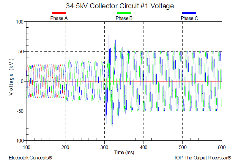
The guidelines in IEEE 1564 advocate computing one or more characteristics from the sampled voltages. From the sampled waveforms in the three phases, such as in Figure 1, one or three voltage magnitudes as a function of time are obtained. For single-channel measurements and multi-channel measurements, the rms voltage is computed over one cycle and is updated every half cycle. This quantity is defined in IEC 61000-4-30 [2] as Vrms(1/2). For three-phase measurements, either the minimum Vrms(1/2) is used to characterize the event, or the “characteristic voltage” is used. These time functions are used to determine the single-event indices retained voltage (“sag magnitude”), depth, and duration [2].
In addition to the two-index method (retained voltage or depth and duration), two single-index methods are introduced in IEEE 1564: the voltage sag energy and the voltage sag severity. In both cases, the severity of each event is quantified by one single value.
RMS Voltage as a Function of Time
From the sampled voltages one or more characteristics as a function of time are calculated for every recording. This function is used to determine the retained voltage and the duration of the event. The rms voltage is calculated over a one-cycle interval, and is updated every half cycle.
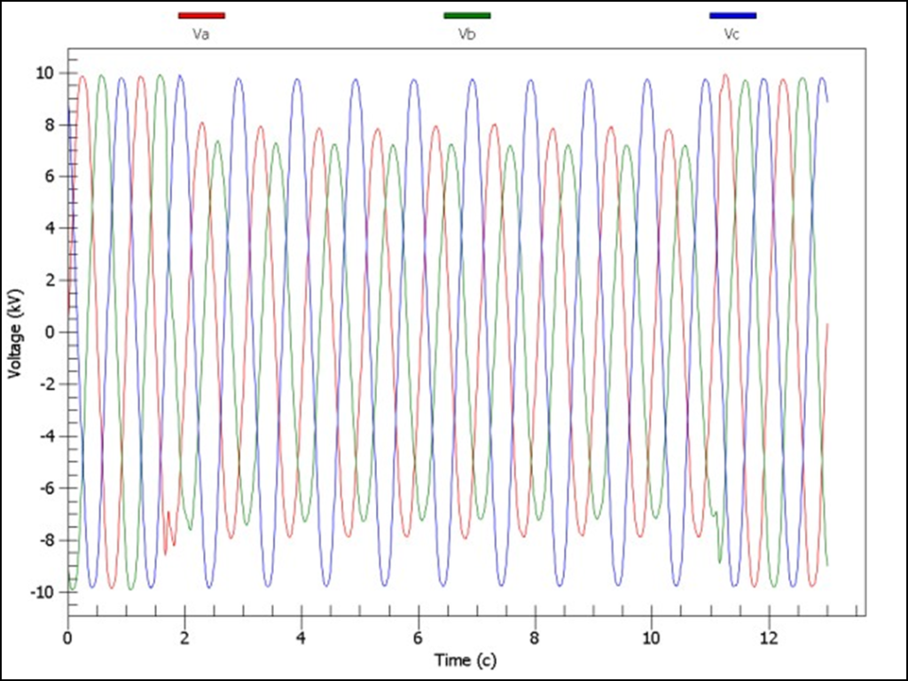
Figure 1: Voltage Sag Example: Three-Phase Voltage Waveform Samples
To calculate the rms voltage, the sampled voltages are squared and averaged over a window with a one-cycle duration, as described in the following equation:

where N is the number of samples per cycle, Vi is the sampled voltage waveform, and k=1,2,3, etc.
IEEE 1564 recommends that the sampling rate be synchronized to the power frequency. That is, the sampling frequency is not a fixed number of samples per second but a fixed number of samples per cycle. This synchronization to the power frequency (also referred to as “phase-locked-loop” or PLL) is essential for the quantification of harmonic distortion and phase angle change calculations. For multi-channel measurements, the rms voltage versus time is calculated for each channel separately.
Retained Voltage and Duration
A voltage sag or voltage swell can be characterized by its duration and its retained voltage. The duration is the time that the rms voltage stays below the threshold. The retained voltage is the lowest rms voltage during the event. Instead of retained voltage, the depth may be used, which is the difference between the retained voltage and a reference or declared voltage.
To determine the sag duration, a threshold setting is needed. This threshold can be defined in multiple ways, such as a percentage of the nominal voltage; a percentage of the long-term average voltage at the location; or a percentage of the rms voltage just prior to the event start. For measurements in low-voltage and medium-voltage networks, the declared or nominal voltage should be used. This value is the most relevant one for the performance of end-use equipment. In low-voltage networks the nominal voltage should be used in all cases. In medium voltage, a different declared voltage may be used to incorporate the primary/secondary ratio of the step-down transformers.
Different threshold values may be used for obtaining the starting and ending instants of the sag. The ending threshold could be higher than the starting threshold by an amount that is referred to as the “hysteresis voltage”. In that case the voltage sag begins when Vrms(1/2) falls below the sag threshold, and ends when Vrms(1/2) is equal to or above the sag threshold plus the hysteresis voltage.
IEEE 1564 recommends the starting threshold be set to 90% of the declared voltage or of the sliding reference voltage. In the event that a different ending threshold is used, the recommended value for the ending threshold is 91% of the declared voltage or of the sliding reference voltage.
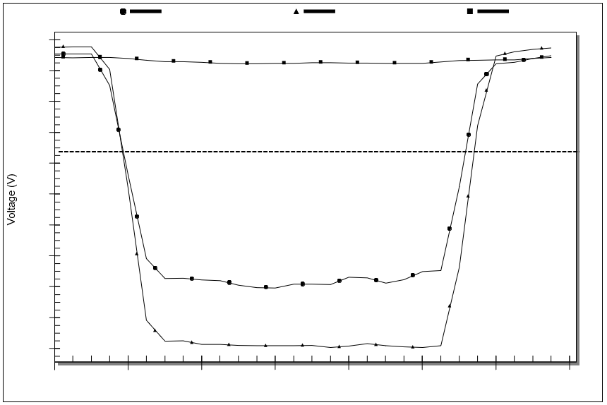
Figure 2: Voltage Sag Example: Three-Phase Voltage RMS Samples with Sag Threshold
Voltage swells can be characterized in the same way as voltage sags. The rms voltage is again used as a characteristic versus time. The single-event indices are the “duration” and the “retained voltage” or “maximum swell voltage magnitude” [2]. The duration equals the amount of time the rms voltage is above the swell threshold. The retained voltage is the highest value of the rms voltage. The recommended value for the swell threshold is 110% of the declared voltage or of the sliding-reference voltage.
Figure 2 presents the rms voltage samples for the voltage sag of Figure 1. The dashed line indicates the voltage sag threshold, which is chosen as 90% of the phase-neutral base voltage of 7.2 kV. If we consider the three phases individually, two phases show a voltage sag of 9.5 cycles duration below the threshold. The retained voltage is 5.21 kV for Phase B.
Voltage Sag Energy and Swell Energy
IEEE 1564 presents voltage sag energy as the energy in the voltage sag event, or the “missing energy” in the voltage waveform. The voltage sag energy is the duration of an interruption that would result in the same loss of energy for a resistive load. The voltage sag energy can also be defined as the non-delivered energy to a resistive load, divided by the rated power of that load. Specifically, IEEE 1564 defines the voltage sag energy characteristic EVS in the following equation:

where V(t) is the rms voltage during the event and Vnom is the nominal voltage.
For voltage sags involving more than one phase, the voltage sag energy is defined as the sum of the voltage sag energy in the individual channels. In case a three- phase approach is used, the voltage sag energy may be calculated from the characteristic voltage as a function of time, with V(t) the characteristic voltage as a function of time.
IEEE 1564 recommends that the voltage sag energy index not be used with short-duration interruptions. A “voltage swell energy” can be defined in the same way as the voltage sag energy.
Voltage Sag Severity
The voltage sag severity is calculated from the retained voltage in per unit and the duration of a voltage sag in combination with a reference curve. Events with longer event duration and lower magnitudes will have larger values of voltage sag severity index. It is recommended to use the ITIC Curve or SEMI F47 curve as a reference, but the method works equally well with other reference curves.
Multi-Channel and Three-Phase Measurements
For multi-channel measurements, the voltage sag magnitude (retained voltage) is the lowest magnitude for the individual phases. The start time of the sag is the time when the rms voltage in one of the phases drops below the sag-starting threshold. The ending time of the sag is the time when all rms voltages have recovered above the sag-ending threshold. The duration is obtained as the time difference between the start time and the stop time. Note that the event may end in a different phase as the one in which it started.
Characteristics Voltage
From the three sampled waveforms in the three phases, a characteristic voltage as a function of time may be obtained. Characteristic voltage is the minimum of the one-cycle, sliding-window rms value of the line-neutral voltage with the zero-sequence voltage removed (VA-V0, VB-V0, and VC-V0) and the line-line voltage (VAB, VBC, and VCA) divided by the square root of three. The lower characteristic voltage is the smallest of the six sliding- window rms voltages. The upper characteristic voltage or PN factor, is the largest of the six sliding-window rms voltages. See Bollen [3] and Sannino et al. [10]
Analyzing the event shown in Figure 2 as a three-phase event results in the characteristic voltage as shown in Figure 3. The lower characteristic voltage has been calculated as the lowest value of the six rms voltages. Like before, the calculation has been updated every half cycle. The resulting duration of the three-phase events is again 9.5 cycles, but the remaining (characteristic) voltage is 4.68 kV or 65% of the nominal phase-neutral voltage of 7.2 kV.

Figure 3: Characteristic Voltage as a Function of Time
SITE INDICES
As input to the site indices, the single-event characteristics are used as obtained from all events recorded at a given site over a given period, typically one month or one year. For the two-index method, a number of alternatives are presented. Each can be summarized as a count of events within a certain range of retained voltage and duration. For single-index methods, the site index is the sum of the single-event indices of all events recorded within the given period.
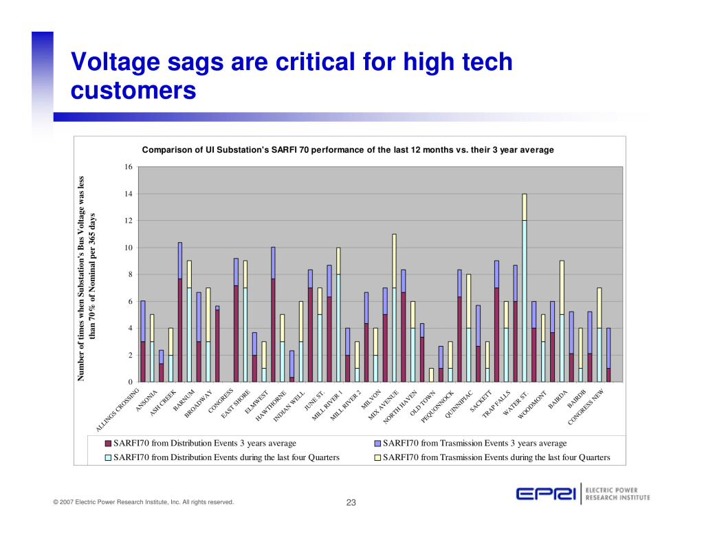
SARFI INDICES
SARFI is an acronym for the System Average RMS Variation Frequency Index. It is a power quality index that provides a count or rate of voltage sags, swells, and/or interruptions for a system. The SARFI index was first described by Brooks in [8]. The size of the system is scalable: it can be defined for a single monitor, a single customer service, a feeder, one or more substations, or an entire power delivery system. There are two types of SARFI indices: SARFI-X and SARFI-Curve.
SARFI-X corresponds to a count or rate of voltage sags, interruptions and/or swells below/above a specified voltage threshold. For example, SARFI-70 considers voltage sags and interruptions that are below 70% of the reference voltage. SARFI-110 considers voltage swells that are above 110% of the reference voltage. Both types of SARFI indices are meant to assess short-duration rms variation events only, meaning that only those events are included in its computation with durations less than the minimum duration of a sustained interruption as defined by IEEE Std 1159, which is one minute [7].
SARFI-Curve corresponds to a rate of voltage sags below an equipment compatibility curve. For example, SARFI- ITIC considers voltage sags and interruptions that are below the lower ITIC curve.
Voltage Sag Tables
A commonly used method of presenting the performance of a site is by means of a voltage sag table. The columns of the tables represent ranges of voltage sag duration, while the rows represent ranges of retained voltage. Each cell in the table gives the number of events with the corresponding range of retained voltage and duration. Each event (that is, each combination of retained voltage and duration) is tabulated in only one cell of the table. Different values are in use for the boundaries between the cells.
Table 1: Voltage Sag Table from IEC 61000-4-11
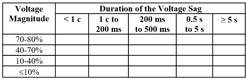
IEEE 1564 presents guidelines on using the voltage sag tables presented by the International Union of Producers and Distributors of Electrical Energy in Europe (UNIPEDE), IEC 61000-2-8, and IEC 61000-4-11 (See Table 1).
Voltage Sag Energy
The sag energy method of characterization uses three site indices: number of events per site; “total lost energy” per site and “average lost energy” per event.
IEEE 1564 presents a Sag Energy Index (SEI), which is the sum of the voltage sag energies for all qualified events at a given site during a given time period. The indices are usually calculated monthly and/or annually. The Average Sag Energy Index, or ASEI, is the average of the voltage sag energies for all qualified events measured at a given site during a given period. When using voltage sag energy indices, IEEE 1564 recommends to not include short-duration interruptions, as one short-duration interruption may have a larger contribution to the index than all voltage sags together.
Voltage Sag Severity
The calculation of site indices for the voltage sag severity method is very similar to the calculation of site indices based on the voltage sag energy. The Total Voltage Sag Severity is the sum of the voltage sag severity for all qualified events at a given site during a given period. The Average Voltage Sag Severity is the average of the voltage swell severity for all qualified events measured at a given site during a given period.
Aggregation
Aggregation in IEEE 1564 refers to the data reduction technique of collecting many distinct measurement components into a single aggregate event for the purpose of computing site and system indices. How the measurements are combined depends on the specific needs of a particular analysis session.
Measurement Aggregation: Many monitoring instruments will record one or more phases during an event. For example, a three-phase voltage sag may result in a meter recording one measurement for each phase. In conducting measurement aggregation, IEEE 1564 recommends representing the multiple phase measurements as only one measurement. A common practice is to choose the voltage channel that exhibits the greatest deviation from nominal voltage. Alternatively, the characteristic voltage, as defined in Section II.F, can be used.
Time Aggregation: The time aggregation is counting a single event if there is a succession of events within a short time, generally caused by a single power system event. An example would be multiple sag events during an automatic reclosing operation. This is the generally accepted practice in indexing voltage sag events. If the customer equipment is impacted by a voltage sag event, it is unlikely that the equipment will be up and running and impacted by a succeeding event during the aggregation time period. Another example is that the survey results that were published in IEEE journals from the EPRI Distribution System Power Quality (DPQ) Monitoring Project used 60-second aggregation time, but the project also explored using 120 seconds and 300 seconds. See Sabin [4] or Sabin et al. [5].
Spatial Aggregation: This refers to finding the worst voltage sags from more than one monitoring point. Spatial aggregation has also been employed when multiple meters are employed to monitor only a single phase of a system. In this case, three meters each monitoring one phase of a feeder can be combined to give the voltage sag performance of the bus supplying the feeder.
When using spatial aggregation to reduce the number of rms variation measurements, the measurements from multiple monitoring instruments are combined into a single measurement. An application is in computing rms variation indices at a single substation that is monitored at multiple buses. Another example is computing rms variation indices for a single industrial facility that is monitored at each service entrance of its supplying feeders. See Dettloff et al. [9].
Monitor Availability
It is not unusual during the course of a monitoring project to experience periods when an instrument is off-line due to instrument calibration or malfunction. Poor data management practices can also result in missing measurements. When combining indices taken from different monitoring sites, it is vital that the total time that each monitor was available is taken into account.
SYSTEM INDICES
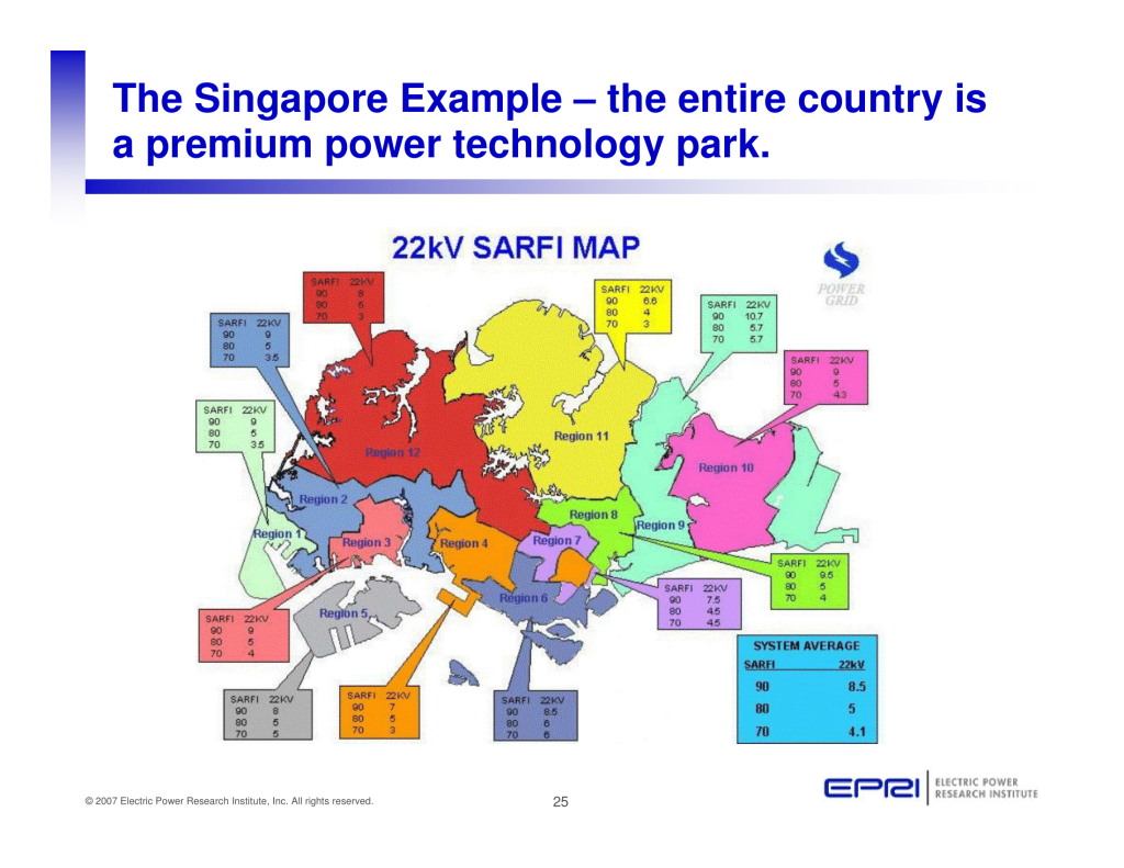
IEEE 1564 includes guidelines on how to compute indices for more than one power quality monitoring site (that is, system indices) from weighted averages or from weighted percentiles. The system indices are defined such that they may be applied to systems of varying size. System indices may be calculated for the whole system operated by a network company; for all networks at one voltage level over a whole country or geographical area; for a group of feeders; etc. Other issues related to system indices presented in IEEE 1564 include site selection, sampling weighing factors, and statistical values.
The SARFI indices for a system are obtained as the average of the indices for the different sites. The SARFI value may be interpreted as quantifying the “average voltage quality” over the whole system or the part of the system being considered. When using SARFI indices to describe individual sites, it is possible to give a 95th percentile to characterize the quality of the whole system.
When voltage sag tables are used, both average values over all sites and 95th percentile values can be used. When average values are used, weighting of the values may be considered. Weighting is also possible when using the 95th percentile, but it is less useful unless a very large number of sites is being monitored. Each element of the voltage sag table should be considered as one index to which the statistical processing (average, 95th percentile, etc.) has to be applied. The resulting table for the whole system does not correspond to any individual site.
When using voltage sag energy indices, system indices are calculated by taking the average value of the site indices. See Thallam et al. [6]. The average sag energy index ASEI for the whole system is obtained by dividing the sum of the site values with the number of sites involved. The system index for voltage-sag severity should be obtained from the site indices in the same way as for the other indices: either as a weighted average or as a 95th percentile.
NEXT STEPS
The next activities of the IEEE P1564 Task Force include promoting the new standard at international conferences. The task force will sponsor a panel session on voltage sag indices at the 2015 IEEE Power & Energy Society General Meeting in Denver, Colorado, USA. Discussion of IEEE 5164 at meetings during two IEEE conferences per year will result in a short- and long-term revision plan. More information will be posted on the task force website: http://grouper.ieee.org/groups/sag/.
REFERENCES
[1] IEEE, 2014 IEEE Std 1564-2014 Guide for Voltage Sag Indices.
[2] IEC, 2008, IEC 61000-4-30 ed. 2.0, Electromagnetic Compatibility – Power Quality Measurement Methods.
[3] M.H.J. Bollen, 2003, “Algorithms for Characterizing Measured Three-Phase Unbalanced Voltage Dips,” IEEE Transactions on Power Delivery, vol. 18, no. 3, 937-944.
[4] D.D. Sabin, 1996, An Assessment of Distribution System Power Quality, Volume 2: Statistical Summary Report. EPRI, Palo Alto.
[5] D.D. Sabin, T.E. Grebe, A. Sundaram, 1999, “RMS voltage variation statistical analysis for a survey of distribution system power quality performance,” Proceedings of IEEE Power Engineering Society Winter Meeting, vol.2, 1235-1240.
[6] R.S. Thallam, G.T Heydt, 2000, “Power acceptability and voltage sag indices in the three phase sense,” IEEE Power Engineering Society Summer Meeting, vol.2, 905-910.
[7] IEEE, 2009, IEEE Std 1159-2009 Recommended Practice for Monitoring Electric Power Quality.
[8] D.L Brooks, R.C Dugan, M. Waclawiak, A. Sundaram, 2008, “Indices for assessing utility distribution system RMS variation performance,” IEEE Transactions on Power Delivery, vol.13, 254- 259.
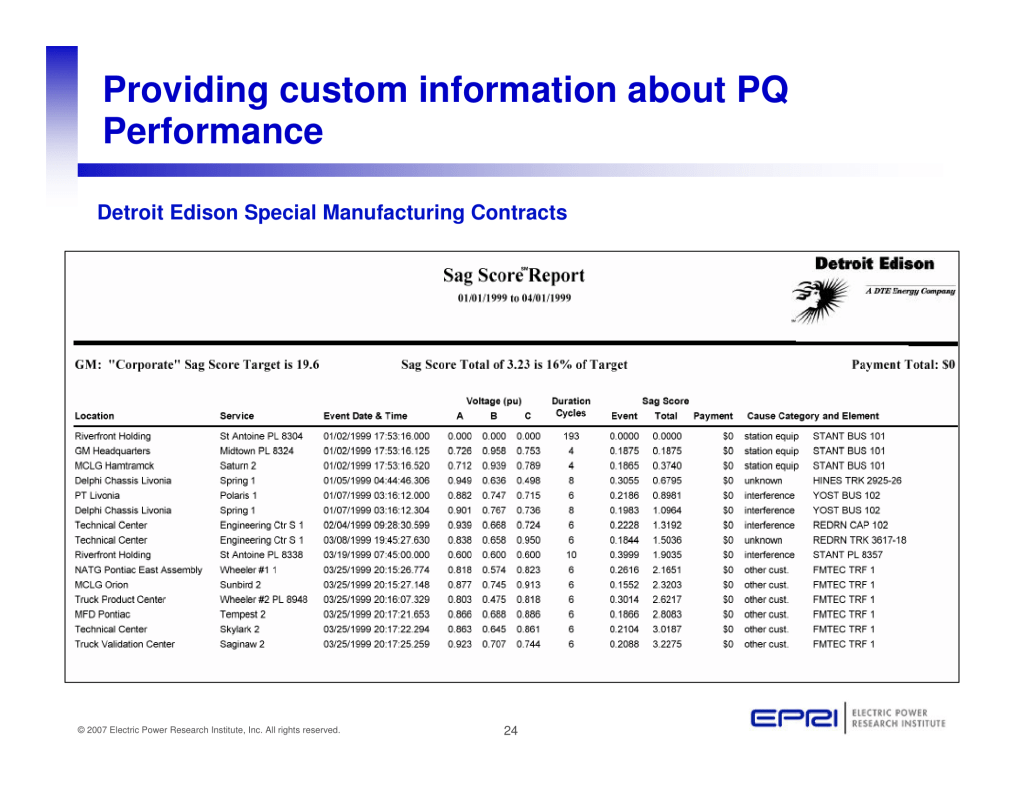
[9] A. Dettloff, D.D. Sabin, 2000, “Power quality performance component of the special manufacturing contracts between power provider and customer,” Proceedings of Ninth International Conference on Harmonics and Quality of Power (ICHQP), 2000., vol.2, no., 416-424.
[10] A. Sannino, M.H.J. Bollen, J. Svensson, 2005, “Voltage tolerance testing of three-phase voltage source converters,” IEEE Transactions on Power Delivery, vol.20, no.2, 1633- 1639.