Voltage Disturbances Flicker Measurement

Published by Zbigniew Hanzelka & Andrzej Bie´n, AGH University of Science and Technology, October 2005

Flicker Measurement Introduction

The power supply network voltage varies over time due to perturbations that occur in the processes of electricity generation, transmission, and distribution. Interaction of electrical loads with the network causes further deterioration of the electrical power quality. High power loads that draw fluctuating current, such as large motor drives and arc furnaces, cause low frequency cyclic voltage variations that result in:

• flickering of light sources which can cause significant physiological discomfort, physical and psychological tiredness, and even pathological effects for human beings,
• problems with the stability of electrical devices and electronic circuits.
  

Figure 1 illustrates the way in which a small voltage change produces a noticeable effect on the luminous flux of a bulb.

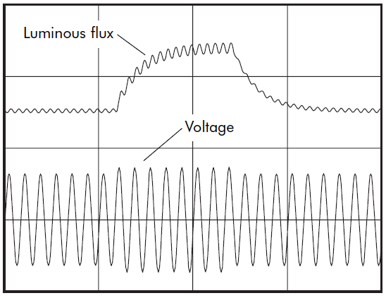
Figure 1 – Change in luminous flux resulting from a temporary voltage change [1]

Recurrent small changes of network voltage amplitude cause flickering of light sources. The effect is popularly referred to as ‘flicker’ and is a significant power quality parameter. An example of a network voltage spectrum where flicker is apparent is shown in Figure 2. The spectrum shown is typical of the voltage of a network supplying a large non-stationary electrical drive. A bulb, supplied from the same node, will flicker with frequency about 1 Hz.

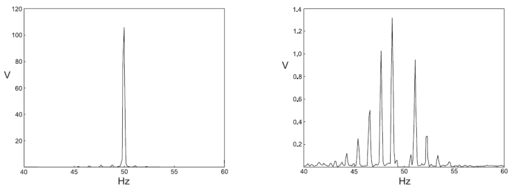
Figure 2 – Power network voltage spectrum; in the diagram on the right the 50 Hz component is omitted

Flicker is expressed in terms of two parameters: short term flicker severity PST and long-term flicker severity PLT. The measurement of these parameters is discussed later in this document.

Estimation of voltage fluctuations

The phenomenon of flickering of light sources has been known since the introduction of power supply networks. However, it grew rapidly along with the increase in the number of loads and the increase in the power consumed. Considerable research has been conducted into the measurement and mitigation of flicker. In order to quantify the scale of light flickering phenomenon research has been conducted with the aims of developing measurement equipment, containment techniques and methods of mitigation. This Section discusses measurement principles and the generic design principles of measurement instruments.

Initially, instrument designs were based on simple observation of luminous flux. The next step was to develop a model of the human reaction – in the form of discomfort or annoyance – to the fluctuation of luminous flux. The model was based on a 60 W, 230 V tungsten bulb, since that was the most commonly used light source in Europe at that time.

Figure 3 shows the threshold of perception of flicker plotted against percentage voltage change (y axis) and frequency of change (x axis). Where the magnitude and frequency of the changes lie above the curve, the effect is likely to be disturbing to a human observer while below the curve it is likely to be imperceptible. The dashed lines represent tungsten bulbs designed for different nominal voltages.

Early flicker measurement instruments included a typical 60 W, 230 V bulb, a luminous flux sensor and an analogue model to simulate human reaction. Following research in the 1980s, activity in the area of flicker evaluation converged and is now centered on the UIE activities. The resulting normalized model instrument is completely electronic; it measures voltage fluctuation and simulates both the response of the light source and the human reaction. Two measurement results are derived; one for short term flicker effect, PST, measured over a ten minute period, and one for long term, PLT, which is a rolling average of PST values over a two hour time frame.

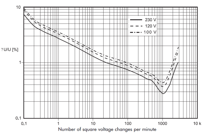
Figure 3 – Flicker perception characteristic for square-shaped voltage changes applied to 60 W bulbs

Measurement of short-term flicker severity

The block diagram of the instrument proposed by the UIE report is shown in Figure 4. The measured voltage fluctuations are processed using a model of the luminous flux versus voltage characteristic of the tungsten bulb and a model of the human reaction to fluctuations of luminous flux. This gives an instantaneous flicker measurement. However, individual people react differently to variations in luminous flux, so the PST value is derived using a statistical model based on experimental work with a large group of individuals.

A detailed block diagram of the instrument is shown in Figure 5. It illustrates the voltage signal processing scheme proposed by UIE and defined in the standardization document [2]. Instruments manufactured according to this document should reproduce the characteristic presented in Figure 3 with uncertainty of less than 5%.

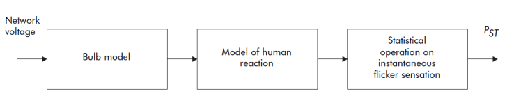
Figure 4 – The operations to determine the flicker severity PST

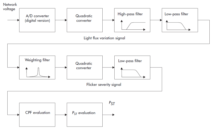
Figure 5 – The structure of the UIE flicker severity measurement instrument

The analogue to digital converter is used only in digital implementations of the instrument. The quadratic converter and the following filters form the model of a 60 W, 230 V tungsten light bulb. The high-pass filter 0.05 Hz serves merely to remove the constant component, since only variations of flux are measured, and the low-pass, 35 Hz, filter represents the dynamic properties of the bulb. The second row in Figure 5 models the human reaction to light flux variations. The reaction of the eye and the brain is modelled with the use of a band pass filter with the following form:

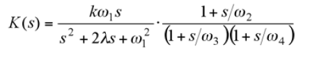
where for a 60 W 230 V incandescent lamp:

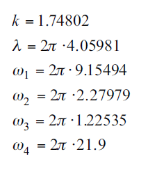
This filter has been designed on the basis of psycho-physiological research on the influence of luminous flux changes on a human being. This research included the analysis of the effect of the frequency and amplitude of the luminous flux changes on human beings. The quadratic converter and 0.53 Hz low-pass filter model the fatigue effect of luminous flux changes.

Figure 6 shows the amplitude response of all the filters used in the instrument.

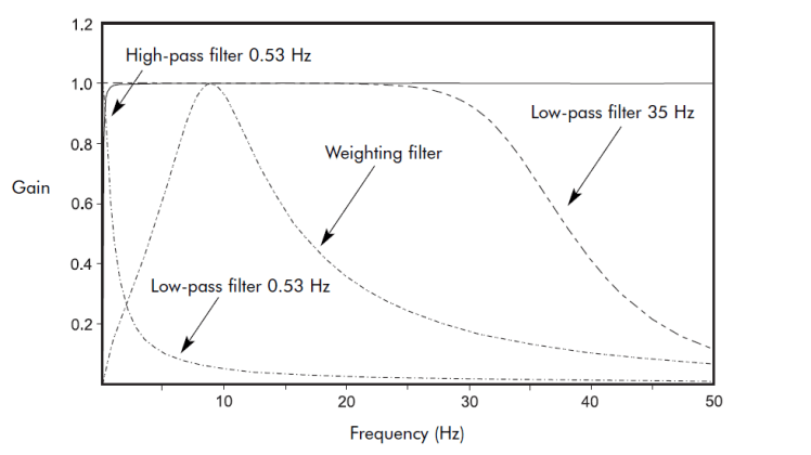
Figure 6 – Amplitude response of the flickermeter filters

The third row in Figure 5 shows the digital statistical processing section. Evaluation of PST is based on the Cumulative Probability Function (CPF) calculation over the observation time. The method of CPF evaluation is shown in Figure 7.

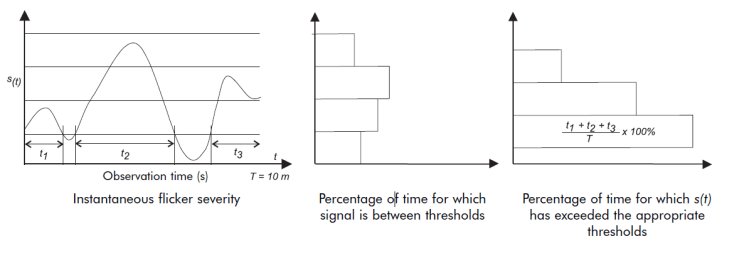
Figure 7 – The process of CPF evaluation

The curve on the left-hand side shows the instantaneous flicker severity (y-axis) plotted against time (x-axis) for the observation period of 10 minutes. The horizontal grid lines represent thresholds that are used to group measurements as shown on the right-hand side. Here the x-axis represents the percentage of the observation time that the discrete instantaneous values exceed the appropriate threshold. (See the example for the lowest group.)

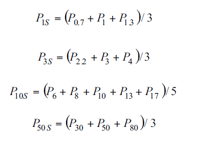
In practice, after samples have been collected for the observation time of ten minutes, the thresholds are set to correspond to percentiles – i.e. so as to have been exceeded for 0.1%, 1%, 3%, 10% and 50% of the observation time of ten minutes. In the following text, these percentiles are denoted as P0.1, P1, P3, etc., while the subscript ‘s’ (e.g. P1s, P3s) indicates that averaging has been applied according to the following formulas:

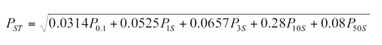
PST is calculated according to the formula:

The PST values are used to evaluate PLT for longer observation times according to:

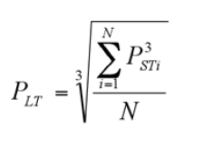
where N is the number of PST periods within the observation time of PLT i.e. 12 PST (10 minutes) measurements would be required to calculate the PLT (2 hours). Figure 8 shows a recording of PST at the network node where an arc furnace has been connected. It can be seen that the operating condition of the furnace influences the PST value. In this case the PST value varies by a ratio of 15:1.

Figure 8 – PST values determined during operation of an arc furnace

Calibration and verification of a flicker severity measuring instrument

Flicker measurement is, as described above, a complex process. If instruments of different design and manufacture are to produce consistent results in the field, correct approval testing and calibration procedures are required.

Approval testing requires validation of the design, e.g. that the accuracy of the modelling and the statistical calculation is sufficiently accurate, by applying pre-determined test signals and monitoring the appropriate outputs. The test signals would be defined in terms of modulation waveshape (sinusoidal or rectangular), amplitude and frequency so that they are consistently reproducible and predictable.

Calibration requires verification of each sample of the instrument, again with pre-determined input signals, to ensure that the indicated result is sufficiently accurate. Manufacturers must indicate how frequently the calibration step should be repeated and provide services to do so.

Measurement and assessment of flicker in the power supply network

As mentioned in the introduction, the basic source of voltage fluctuations (and the consequential flickering of light sources) is large electrical loads.

The mechanism is illustrated in Figure 9.

The voltage at the point of the load connection is less than the source voltage because of the voltage drop

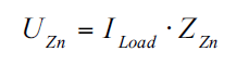
where:

as seen from the points of the load connection (a, b).

Since the voltage at points (a, b) is

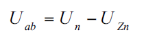
it may be noticed that any ILoad current change, particularly in the reactive component, will cause an undesirable change in the voltage Uab.

In a real power network this phenomenon is much more complex, but the principle is valid.

Often, the question arises as to whether the planned connection of a load to the network would cause flicker or increase the level of flicker above the prescribed limit. The answer to this question depends on the parameters of the power network and any connected loads that may cause negative effects on it.

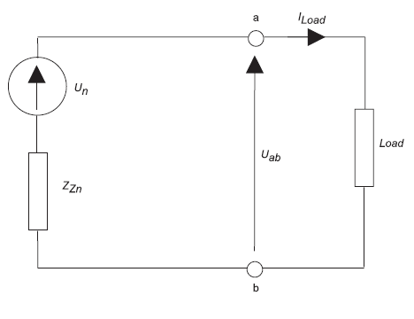
Figure 9 – Influence of a load on a network

Since the effect cannot be measured in advance of connection, the effect must be estimated. Compatibility issues are dealt with in standardisation document IEC 61000-3-3 [5], in which a reference source impedance  equivalent to Re() = 0.4Ω and Im() = 0.25Ω at 50 Hz is assumed.

Additionally, the standard provides a method of improving the assessment by taking account of the profile of the modulation of the supply voltage – i.e. the calculations assume the worst case square form modulation and will therefore require modification for other shapes.

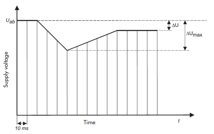
Figure 10 – Example of a load profile from [5]

Figure 10 shows one profile, typical of a motor drive, from [5] showing how voltage changes ΔU are determined for the calculation of d = ΔU/Uab . Values of equivalent step parameters depend on t1, t2, t3 etc, as illustrated in the standard. The calculation of the effective value of voltage is performed every half cycle.

The standard [5] requires that:

• the value of the short-term light flicker severity index: PST ≤ 1.0
  
• the value of the long-term light flicker severity index: PLT ≤ 0.65
  
• stationary relative voltage change: d ≤ 3%
  
• maximal relative voltage change: dmax ≤ 4%
  
• the d value during the voltage change should not exceed 3% for a duration longer than 200 ms.
  

result of manual switching, then the allowable values are increased by 33%. It is important to note that a constant network voltage is assumed, i.e, that without the presence of the load under test, there would be no voltage fluctuations on the power network.

The phenomenon of flicker severity is not additive – mathematical operations cannot be performed on the results of PST or PLT measurements.

Conclusion

Flicker has been a problem in electrical networks from their inception. Since the 1980s, progress in understanding the phenomenon and the process of perception has led to standardisation of measurement methods and instruments to allow flicker to be measured reliably. Modern instruments, employing fast digital signal processing techniques, now allow flicker problems to be rapidly evaluated and resolved.

References:

[1] Guide to Quality of Electrical Supply for Industrial Installations, Part 5, Flicker and Voltage Fluctuations, Power Quality Working Group WG2, 2000.

[2] IEC 60868, Flickermeter, Functional and Design Specifications, 1986.

[3] IEC 60868-0, Amendment 1, Flickermeter, Functional and Design Specifications, 1990.

[4] IEC 61000-4-15:1997, Electromagnetic Compatibility (EMC) – Part 4: Testing and Measurement Techniques – Section 15: Flickermeter – Functional and Design Specifications.

[5] IEC 61000-3-3:1995, Electromagnetic compatibility (EMC) – Part 3: Limits – Section 3: Limitation of Voltage Fluctuations and Flicker in Low-voltage Supply Systems for Equipment with Rated Current ≤16A.

[6] Mombauer W: EMV Messung von Spannugs-schwankungen und Flickern mit dem IEC-Flickermeter, VDE VERLAG, Berlin und Offenbach 2000.

Source:

• Power Quality Application Guide. Voltage Disturbances Flicker Measurement 5.2.3
  
• http://copperalliance.org.uk/uploads/2018/03/523-flicker-measurement.pdf