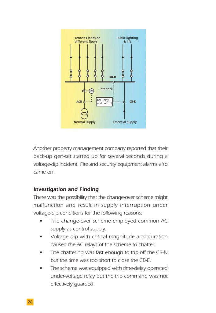
Published By Terry Chandler Director of Engineering, Power Quality Thailand LTD/Power Quality Inc., USA. January 2009
Emails: terryc@powerquality.org, terryc@powerquality.co.th
The Need for Harmonic Modeling and Mitigation in Generator Applications: A Conversation and Guide
White Paper 08-03-2021
Published by Michael McGraw, USA National Sales Manager, Mirus International Inc.,
Introduction & Structure
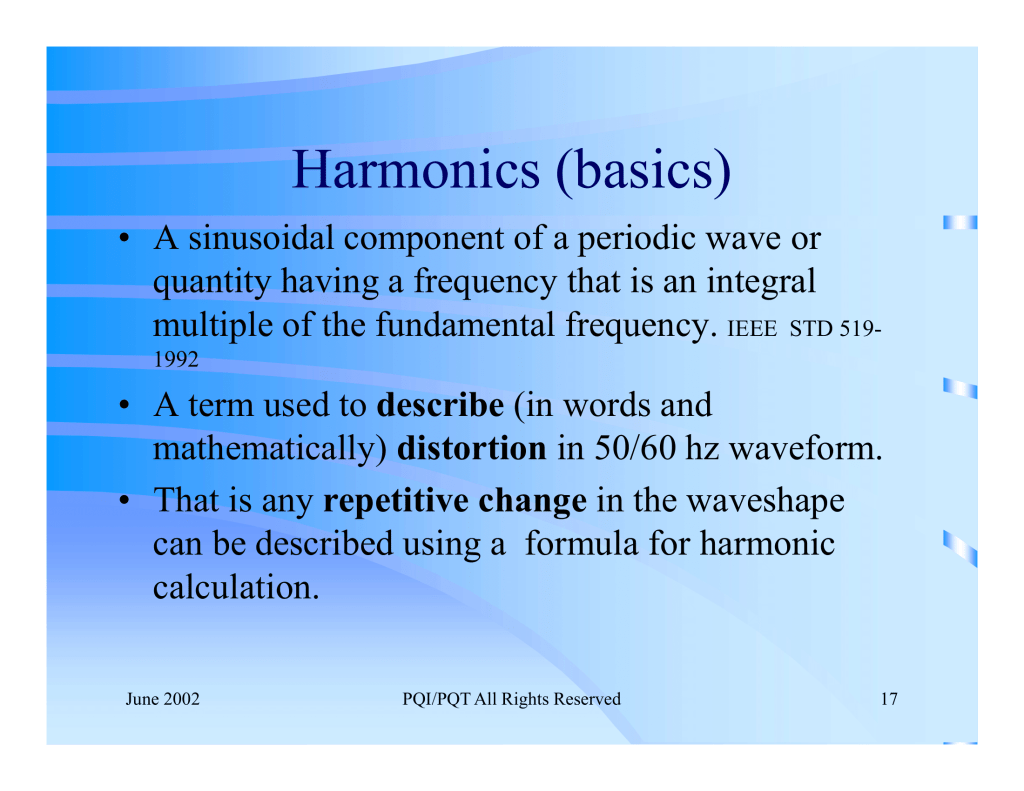
It is widely accepted that performing harmonic studies for non-linear applications is important to ensure a workable and energy efficient installation. It is also accepted that these harmonic studies be performed under normal source conditions and maximum operating load. But it is even more critical to perform harmonic modeling and evaluation under unusual or emergency operating conditions, such as when supplied by a backup Generator source.
Generator sources have a much higher source impedance in comparison with Utility Distribution sources, meaning the short circuit ratio of the overall system is lower. A higher source impedance and lower short circuit ratio will result in a weaker or less stiff overall system, making control of source voltage regulation more difficult, and leading to higher associated voltage distortion from any given current harmonic load condition. Based on this, it is imperative that if a normal Generator Source or Emergency Generator system exists within a distribution scheme, a credible harmonic solution must be modeled, designed, and implemented for this operating configuration. Credible should be defined as a harmonic design that resolves the current harmonic and voltage distortion challenges within the system while not creating operational challenges for any potential source or load package within the circuit.
These challenges would include over- or under-excitation, excessive load voltage boost, excessive load voltage drop and potential resonance between the source and the capacitive reactance of any proposed harmonic mitigation solution. So, we must model and design the circuit to resolve the load current harmonic profile without compromising the operational integrity of the Generator Power Source.
This conversation is broken into two sections, the first is the required information and base data to build the harmonic model and enter this information into a computer simulation software package. The second is a case study on how the comparative modeling was used to analyze filtered versus unfiltered scenarios with Utility and Generator Sources with a provision for a future non-linear load expansion. We will utilize Mirus’ SOLV computer simulation software since it is simple to use and allows for analysis under ‘real world’ conditions, including source/background voltage distortion, Vd, and systemic voltage imbalance. These two factors allow for a true determination of harmonic condition and must be considered to fully understand their impact on the circuit. SOLV software is a free download and is available at
https://www.mirusinternational.com/register.php?reg=1
Part 1: Determining Required Information and Model Data Input
Required Generator Information:
To properly model a source Generator you must know the following data from the Generator specification sheet in order to setup the model:
- kW/kVA rating
- Power Factor
- Unsaturated Sub-transient Reactance (X”d)
- Source Voltage Distortion (when available)
- Source Voltage Imbalance (when available)
This information can typically be found from the Generator Data Sheet. Below is a diagram on how to load the data into the Mirus SOLV software package:
Source Data Graphic: By clicking on the source emblem, the window for source data will open.
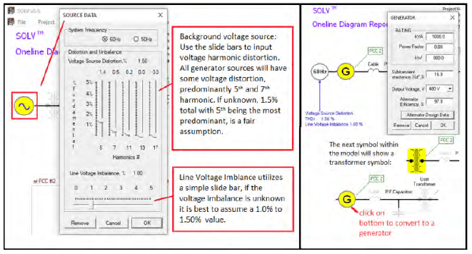
Within the Generator data section, enter the data from the generator specification info. There is a provision for alternator design data, where you can custom load the data. The software is using a “typical” core loss/resistance/reactance model. Care should be exercised when entering custom alternator information.
Required Load Data:
Often there is no load shedding associated with operation on a generator source, but within some Emergency Generator applications, there may be load shedding during transfer. Consult the load schedules and specifications for clarification.
The information below is required for an accurate model:
- Linear Load information including an estimate of the Displacement Power Factor. Consult the load schedule if present within the specification and drawings. For retrofit applications, a site survey should be done. Keep in mind that not all branch circuits are fully loaded, so a survey of the breaker current ratings is not appropriate. Linear load data will affect ITHD calculations at the Point of Common Couplings (PCC 1 and PCC 2) but will have minimal, if any, effect on VTHD. Including them is not always necessary for an accurate depiction of the effect of harmonic distortion.

Non-Linear Load Information includes all existing drive loads and anticipated new drive loads associated with the review. The following data should be collected:
- Drive Configuration: This would include the types of ASD/VFD equipment present within the system.
- Drive Topology, such as 6 pulse or phase shifted multi-pulse.
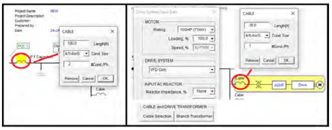
- Secondary/DC bus impedance structures, such as line reactors and/or DC bus inductors.

- Anticipated Load Values: Current Harmonic output of a VFD is a function of its relative load level. That is, the actual current load is relative to the rated load. For the SOLV simulation we use a Load %, not a speed reference within the model.

For worst case scenario, it is best to model the most heavily loaded condition anticipated. This may not always be 100% but selecting 100% would result in the highest levels of voltage distortion.
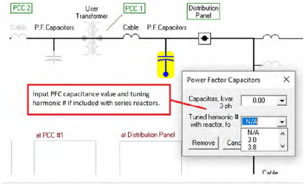
Cable runs and Power Factor Correction:
Within the SOLV Modeling software, you can input individual branch circuit cable runs or primary circuit cable runs for a more accurate representation of overall circuit impedances. This will result in slightly lower ITHD and VTHD values at the PCC’s but can be neglected for worst case scenario, if unknown. Another important consideration is any existing or proposed power factor correction that may be within the circuit. If power factor correction capacitors exist, they should be included so that their impact on power system resonance is taken into consideration. Adding Power Factor Corrective equipment to a high harmonic load structure increases the possibilities of triggering harmonic resonance, especially on weak source systems like a generator supply. Within SOLV, you can add PF correction into the model and qualify the construction should it be of a tuned or detuned configuration.
To enter information on cable runs, see the diagram below. Keep in mind, the secondary impedance structure of associated cabling within the distribution system can have an effect. For the highest simulation accuracy, cable details should be included. But, if cable details are not available or if you want the model to be conservative in nature, you can ignore the cables or only include some runs of conductors. If the modeling is done without these secondary impedance structures, actual results will tend to be marginally better than the model itself. See diagram below for two cable run input locations within the SOLV software.
Part 1 Summary: Building the model may seem complicated but it is normally relatively simple. The entire concept and the ease of running these models is best demonstrated via the Case Study in Part 2. Even complicated systems can be reviewed relatively quickly by organizing the data properly and building a good base model. Then variations as to constructions and operating scenarios can be made with simple changes to the model data, including source parameters and future load structures.
When possible, it is important to include the following within the harmonic model:
- Source power quality condition is of an overriding concern when reviewing true harmonic conditions. If data is available relative to source or background voltage distortion or systemic voltage imbalance, it is best to include it within the model. If this information is not available, a good ‘rule of thumb’ is to assume 1.5% to 2% Background Vd for most commercial applications, 2% to 3% for moderate industrial applications such as Water/Waste-Water installations, and 5% or greater for heavy industrial installations such as Oil & Gas production. Systemic Voltage imbalance should be included based on actual test data or estimated at around 1% if unavailable.
- Of course, non-linear load values should be considered. Software, such as SOLV, that calculates the harmonic spectrums of the loads through discrete components and does not depend upon look up tables structured around full load models, will provide the most accurate simulations. VFD speed and % load are different variables. The relationship between speed and % load is not linear since the motor load torque requirements can and will dictate the drive current draw characteristics.
- If the circuit contains existing power factor correction equipment, it must be reviewed and included within the model. Make sure to determine if the PFC assemblies are tuned, and at what frequency. Non-tuned PFC’s can have serious resonance consequences to the voltage distortion within the system.
Part 2: Case Study: Temple TX Membrane Treatment Expansion
To understand the need and format of the harmonic mitigation modeling in relationship to a Generator Back-up (B/U) project, the following case study can be reviewed. For this discussion, we will review one Utility-B/U Gen-Set grouping to simplify an already complex analysis. The site actually has four Utility sources feeding isolated load structures, each having their own back-up generation. These were all analyzed for the project demonstrating the capabilities of this approach to harmonic analysis.
Step 1: One Line Review:
The first step is to review the 1-lines to gain a general sense of the situation. This particular project was complicated since it involved multiple Utility feeds/Backup Gen-set sources, within multiple load sections of the project. One part of the overall 1-Line is shown below:

Note that there is no direct tie-breaker between the two Utility services and that the MCC loads are normally fed through the first Utility service, but are also fed from Gen-Set 1 when in standby mode. These types of supply changes must be considered when building your harmonic model. Also of interest is that there is 1200 HP of VFD loads potentially being fed from a 1500 kW generator on each side of the 1-line, with an additional 400 HP to be added at a future date. This needed to be considered within the sizing of the Gen-Sets, and construction specification for the harmonic filters, both existing and future. In this example, Utility source and Gen-set sources were both modeled to allow a complete project prospective.
Step 2: Modeling the Source
To model the Utility Source, a quick review of the nameplate or specification sheet of the transformer should be your first step. You will need to confirm the kVA, power factor, and % Impedance of the transformer. You should also review the Utility voltage, Available Short Circuit (ASC), Source Voltage imbalance and Source Voltage Distortion.
Utility Supply: 12.47 kV to 480V, 1500 kVA, .80 pf transformer. We were not given the ASC, or source condition. To be conservative, we assumed a 3kA ASC at 12.47 kV, 1% Voltage imbalance, and 1.5% Background Vd for the source.
Generator Supply: 1500 kW, 480V, 0.80 pf, X”d = 16%. No voltage imbalance or background voltage distortion was provided so the same assumptions were made as per the Utility Supply.

Utility Source Model Construction

Backup Generator Source Model Construction
Step 3: Building the Load Profile
For Utility Source – B/U Gen-Set 1, a quick review of the linear versus non-linear loads should be your first step.
Non-linear Load Profiles:
- (Qty 3) 400 HP VFD’s with Harmonic Filters – Pump 2, 3 and 4: Since the VFD’s are being used for speed regulation, the actual maximum load current anticipated on each drive will be less than full load. The SOLV software versus other manufacturer and commercial harmonic software products takes this into consideration when calculating the current harmonic injection into the source impedance. Many other software packages will use the full speed spectrum which may not be accurate for a partially loaded VFD structure. For this example, we will use a 70% loading nominal value on all three VFD’s for the evaluation.
- (Qty1) 400 HP Future VFD Load: Pump 1. The project calls for a fourth future designated 400 HP pump. Therefore, for a worst case scenario, analysis was done with all four pumps operating.
Linear Load Profile: From the 1-Line, Linear Load profiles were estimated as follows:
- MCC-1: 600A at a nominal loading of 40% -> 240A @ 480V = 200 kW, pf of .95 Primary MCC:
- 800A at a nominal loading of 40% -> 320A @ 480V = 265 kW, pf of .95 (Note: there are AC Unit Condensers present in this case they are linear loads)
Total Linear Load for the model: 465 kw

Note: No cable runs and no specific detail on the VFD’s are known since this is a new installation and the drive brand and construction are unknown.
Step 4: Models to Compare Performance to IEEE Std 519 under Different Source Conditions
This step is quite easy. First build a base model using the Utility Source data with the associated loads without any harmonic mitigation or filtration. The model should reflect line reactors and/or DC link inductors should that be the normal installation configuration from the manufacturer. This will act as your base model and help streamline the modeling function moving forward. For this study, I have labeled this as the Utility Source – Unfiltered (Model 1). Then I can simply save this model and as variations are made, the new files can be saved under different file names. SOLV also allows comparative models in one file by establishing a base model as “Scenario A” and then adding a second scenario “Scenario B” for comparison.
It should be noted that the SOLV software only has built-in models for Mirus AUHF and AUHF-HP passive harmonic filters. These models are based on our proprietary inductive /capacitance network and therefore, the use of SOLV is not appropriate for modelling competitive passive filter products. An important difference in the Mirus filter design is our low capacitive reactance ratio to full power rating, which prevents overexciting a generator supplied circuit. At 100 HP and greater power, the kVAR to kW ratio is less than 15%. For competitive filters, this ratio can be as high as 40%, which can result in higher voltage boost at no load, generator instability and the requirement for a capacitor switching contactor. As stated, the SOLV software is not appropriate for modeling any passive filters other than the Mirus product offering.
Following are the Model Summaries we will review:
- Model 1: Utility Source with 3% AC Reactors
- Model 2: Utility Source with Mirus AUHF Filters
- Model 3: Generator Source with 3% AC Reactors
- Model 4: Generator Source with AUHF filters
- Model 5: Generator Source with AUHF-HP High Performance filters
It is noted that IEEE519 defines the limits at the Point of Common Coupling (PCC). For reliable equipment operation, we recommend that the analysis consider the Generator terminals to be the PCC when operating on the Generator supply.
Model 1: Utility Source – Unfiltered
Loading the Data as previously discussed, we input the Utility parameters and then input the step-down transformer information as the User Transformer. This allows us to compare the Utility PCC 2 versus the End User PCC 1 within the model:
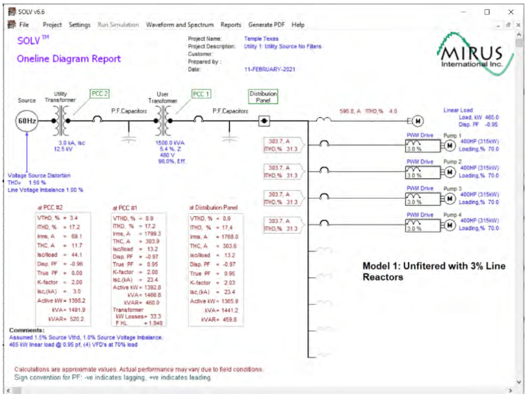
As can be seen, on Utility supply at PCC 1, the 480V VTHD level is 8.9% and ITHD or ITDD is 17.2%. In this case, ITHD and ITDD are the same value because the analysis was done at what is anticipated to be maximum load level. At the 12 kV Utility bus, PCC 2, VTHD is 3.4%. ITDD is the same as the PCC 1 ITDD since these harmonic currents pass through the transformer. The IEEE 519 compliance schedule, showing both 1992 and 2014 requirements, is below:

Model 2: Utility Source Filtered with Mirus AUHF Filters
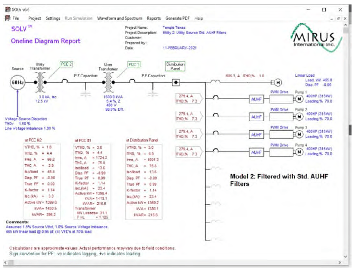
Once we filter the VFD’s, the associated harmonic distortion is reduced at PCC 1 to 3.0% VTHD and 4.4% ITHD. This indicates that the harmonic filtration limited the net PCC 1 voltage distortion to only 1.5% more than the background Vd from the source (1.5%). As per the following tables, IEEE 519 limits are met at both PCC 1 and PCC 2.

The model and results show that there is significant headroom for future non-linear load additions without concern for exceeding harmonic compliance.
Model 3: Generator Source with 3% AC Reactors
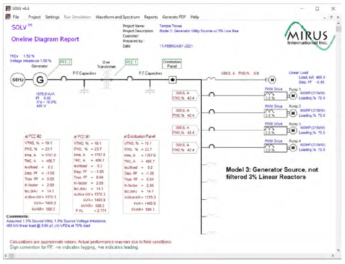
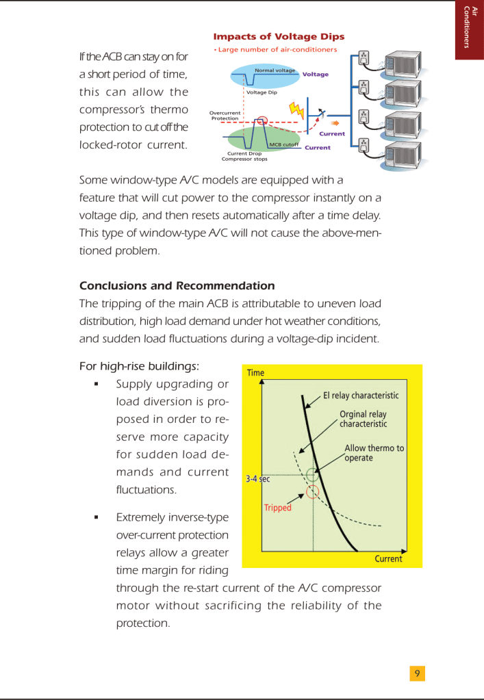
As can be seen, the weak Generator Power Source has a significant effect on the harmonic profile of the circuit. At PCC 1, Vthd is projected to be 19.1% and Ithd 23.7%. This dramatically shows the need to run Back-up Generator harmonic modeling. The IEEE 519 compliance schedule is as follows:

It is clear that operating the pumps with only 3% AC reactors exhibits poor harmonic performance, to the point where it is doubtful that the generator would function properly due to voltage regulation challenges and overheating of the alternator windings.
Model 4: Generator Source with AUHF filters


With respect to voltage distortion, the 8% 2014 version limit is met but the previous 1992 version limit of 5% is not. So the question becomes what level of voltage distortion is acceptable for the application. With respect to current distortion, we see that the lower limits defined by the low short circuit ratio are marginally exceeded in both total ITDD and for the largest individual harmonic, which is the 7th harmonic in this case.
Step 5: Additional Mitigation Model with AUHF-HP Filter Option
Since IEEE Std 519 compliance is not fully met when supplied by generator source even when the standard harmonic filter is applied, a final simulation is done using higher performance AUHF-HP harmonic filters.
Model 5: Generator Source with High Performance AUHF-HP filters

With the additional harmonic mitigation capabilities of the HP series AUHF filter, the overall VTHD and ITHD are both reduced to less than 5%. Since this is a conservative analysis, we can safely predict that all requirements of IEEE Std 519 will be met in both Utility and Generator Source configurations even when all four pumps are in operation. IEEE compliance summary is below:

Final Design Summary and Conclusions:
Below is a summary of the models for this case study:
| Model | Configuration | ITHD | VTHD | kVAR | Total pf | IEEE |
|---|---|---|---|---|---|---|
| 1 | Utility Source with AC reactors | 17.2% | 8.4% | 460 | 0.95 | IEEE 519 Fail |
| 2 | Utility Source with Std. AUHF Filters | 4.4% | 3.0% | 216.6 | 0.99 | IEEE 519 Pass |
| 3 | Generator Source with AC reactors | 23.7% | 19.1% | 506.3 | 0.94 | IEEE 519 Fail |
| 4 | Generator Source with AUHF filters | 5.7% | 5.8% | 156.1 | 0.99 | IEEE 519 Marginally Fail |
| 5 | Generator Source with AUHF-HP filters | 4.3% | 4.9% | 145.1 | 0.99 | IEEE 519 Pass |
- All measurements shown are at PCC #1
- Note the dramatic reduction in Reactive Power Consumption and Power Factor Improvement when harmonic mitigation is applied to the circuit.
- The computer simulations confirmed that IEEE Std 519 requirements would not be met with the application of reactors only, especially under Generator supply.
- With the application of standard Lineator AUHF passive filters, IEEE Std 519 was met under Utility supply but marginally failed under Generator supply. The application passed VTHD limits for the 2014 edition, but slightly failed on current. This could be considered acceptable performance since it is highly unlikely that these levels would cause equipment malfunction.
- A final simulation was performed using higher performance Lineator AUHF-HP filters which guarantee < 5% ITDD. In this simulation, all requirements for both 2014 and 1992 editions of the standard are met.
- An interesting observation is the reduction in Reactive Power Consumption as harmonic mitigation is applied. Reactive power is non-work producing power, meaning that the overall system is becoming more efficient as a result of the harmonic mitigation strategy.
- Once the VFD supplier is determined for the project, a revamp of the harmonic models for the VFD configuration is advisable to help fine tune the evaluation. Variables that should be considered were discussed within Part 1 of the paper. The successful bidder will be required, by specification, to provide a harmonic review of all segments of the project, which include Source Voltage Distortion and Voltage Imbalance as a modeling qualification.
- As part of the specification, the supplier of the equipment will be required to perform verification of harmonic performance and compare these results to the selected harmonic mitigation manufacturer’s required harmonic models. The successful manufacturer and contractor must warranty their harmonic performance to IEEE Std 519, through modeling and field verification.
The need to Model Harmonics in relation to the IEEE 519 Std under Generator Supply is paramount to a sound engineering design if a Generator is an available source for the loads.
The Need for Harmonic Modeling and Mitigation in
Generator Applications: A Conversation and Guide – White PaperDownload
Generator Applications: A Conversation and Guide – White PaperDownload
Contact
MIRUS International Inc. 31 Sun Pac Blvd., Brampton, Ontario, Canada L6S 5P6
Call: 1-888-TO MIRUS or 905-494-1120 Fax: 905-494-1140
Email: mirus@mirusinternational.com
Power Quality Standards Overview (2002 to 2020)
Published By Terry Chandler Director of Engineering, Power Quality Thailand LTD/Power Quality Inc., USA. June 2002
Emails: terryc@powerquality.org, terryc@powerquality.co.th


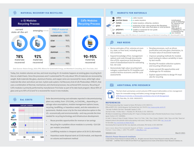
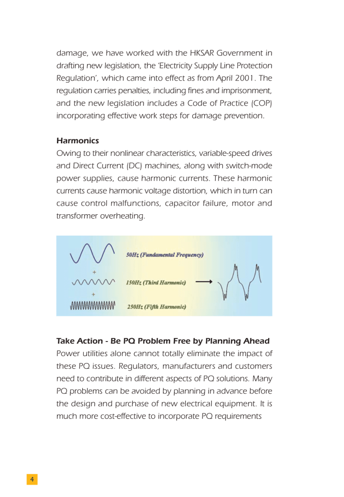
SOLAR PHOTOVOLTAICS END- OF-LIFE MANAGEMENT

Published by EPRI (Electric Power Research Institute), March 2021

PG4400 Capture of PF Capacitor Switching Transients an Intelligent PQ Instrument
Published By Terry Chandler Director of Engineering, Power Quality Thailand LTD/Power Quality Inc., USA. April 2007
Emails: terryc@powerquality.org, terryc@powerquality.co.th
Calculate Neutral Current in Dran-View 7
Published By Terry Chandler, Director of Engineering, Power Quality Thailand LTD/Power Quality Inc., USA. March 2021. Emails: terryc@powerquality.org, terryc@powerquality.co.th
Application note to calculate neutral current in DV7 or manually from RMS values manually and automatically with DV7 Enterprise math channels!
The neutral current in a three-phase, four-wire wye system represents the imbalance of the three-phase conductors, also known as the “hot” conductors. If the three hot conductors are equal, as in the case of supplying a three-phase motor, and if there is no imbalance and the neutral current is zero. In a single-phase system, the neutral carries only the imbalance of the two hot conductors, an easy calculation. However, in a three-phase wye system, even if only two of the three phases and the neutral run a single-phase load, you must use the neutral formula.
Step 1
Note the neutral formula. If A, B and C are the three phase currents, the formula to find the neutral current is the square root of the following: (A^2 + B^2 + C^2 – AB – AC – BC).
Step 2
Use example phase currents of five amps, eight amps and 10 amps. Square each of the phase currents and add the total of the three numbers. Using these examples, the squared numbers are 25, 64 and 100. The sum of these numbers is 189.
Step 3
Subtract each multiplied pair of numbers from the current total. AB, or five multiplied by eight, is 40; AC, or five multiplied by 10, is 50; and BC, or eight times 10, is 80. The total of these numbers is 170. This number subtracted from 189 leaves 19.
Step 4
Take the square root of the calculated number. The resulting number is the neutral current. The neutral current in the example is about 4.36 amps.
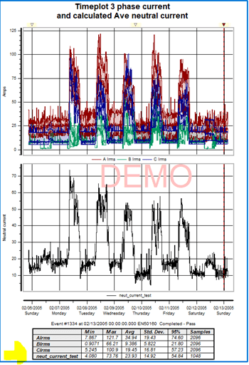
Using DV7 to automatically calculate the neutral current, i.e. a virtual neutral channel. Below is a example of the Neutral current calculated by this formula and displayed in DV7.
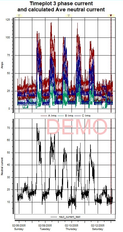
Figure 1 – Example of a neutral current
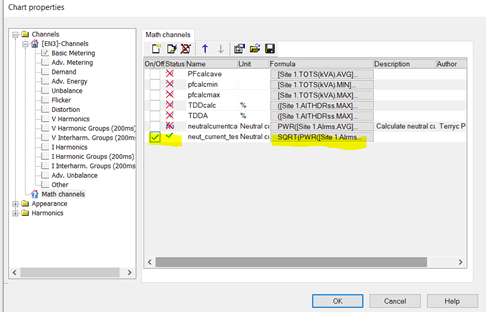
Select the Math Channels as shown below and select new (in the red circle)
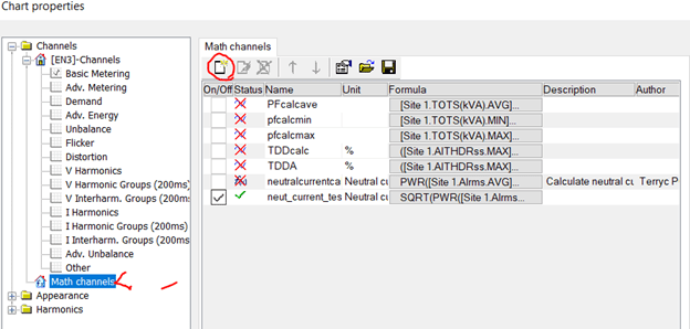
Below is the math channel screen to enter a new channel definition.
Note: this is for advanced users of DV6 or DV7 and the entering the formula can be challenging until you learn the exact structure required. It does alert you to typing or formula format errors.
The procedure for entering the formula is in the steps below:
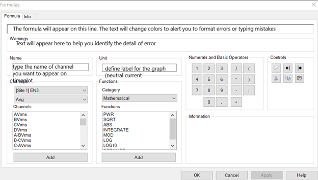
- Enter the name of this channel (neutral current cal)
- Define the units neutral amps
- Select the datafile you want the math channel to use for values
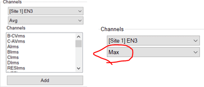
5. Select the parameter you want in the formula. For this example, The formula requires use to square the currents ,we can chose to use the max, min or Average from the DV7 channels. I recommend Avg, unless you are looking for the absolute maximum neutral current then use the Max
6. Next we start to enter our formula
Note the neutral formula. If A, B and C are the three phase currents, the formula to find the neutral current is the square root of the following: (A^2 + B^2 + C^2 – AB – AC – BC).
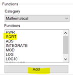
7. Select SQRT from the math function followed by Add:
8.
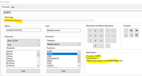
Note DV7 provides the information about function and what it needs. It also warns the formula is not functional at this time. (remember your 1st year algebra 😊)
9. Next carefully add the parameters as shown (or copy this string and paste in the formula window
SQRT(PWR([Site 1.AIrms.AVG];2)+PWR([Site 1.BIrms.AVG];2)+PWR([Site 1.CIrms.AVG];2)–[Site 1.AIrms.AVG]*[Site 1.BIrms.AVG]–[Site 1.BIrms.AVG]*[Site 1.CIrms.AVG]–[Site 1.CIrms.AVG]*[Site 1.AIrms.AVG])
10. <if you are typing it in, pay close attention to copy the punctuation and syntax exactly or you may enjoy some time debugging your first math channel experience>
It should look like this when you are finished. Note: The pink color is DV7 way of saying “Good job it should work.
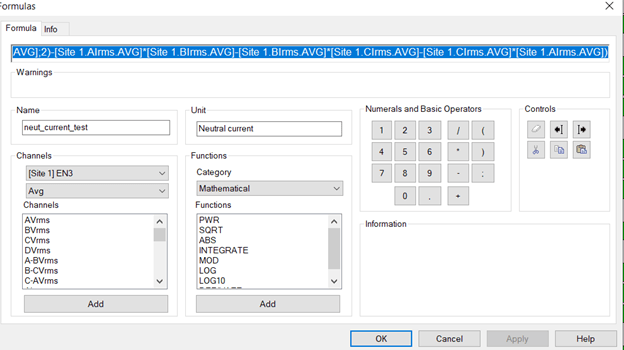
Copy the text below into the math channel (duplicated for your records)
SQRT(PWR([Site 1.AIrms.AVG];2)+PWR([Site 1.BIrms.AVG];2)+PWR([Site 1.CIrms.AVG];2)–[Site 1.AIrms.AVG]*[Site 1.BIrms.AVG]–[Site 1.BIrms.AVG]*[Site 1.CIrms.AVG]–[Site 1.CIrms.AVG]*[Site 1.AIrms.AVG])
Next step is to save you work. DV7 double checks it for errors and saves it as shown below.
It will remain in your DV7 application until you delete it or reinstall a new DV7.
In the screen below you can select to turn on/off you math channels like any other channel.
Also note: the new Neutral current channel can be characterized like any other parameter channel in DV7. Below is shown with the statistical values:
For more information on Dran-View 7 software. You can visit:
Dran-View 7 Blog Post
Dranetz Dran-View 7 Software
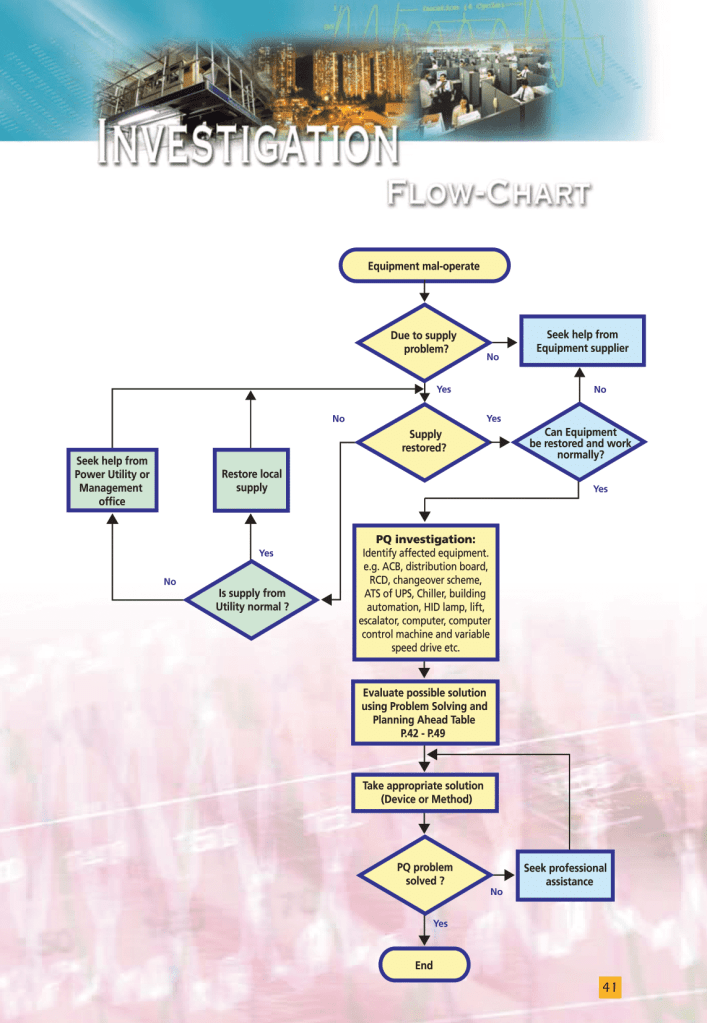
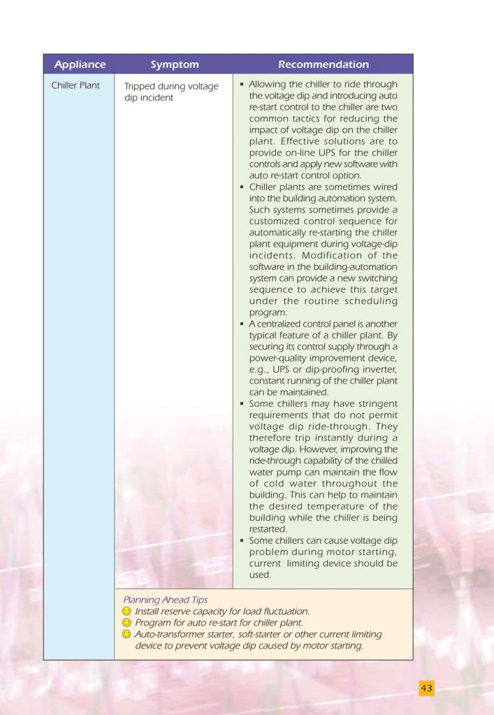
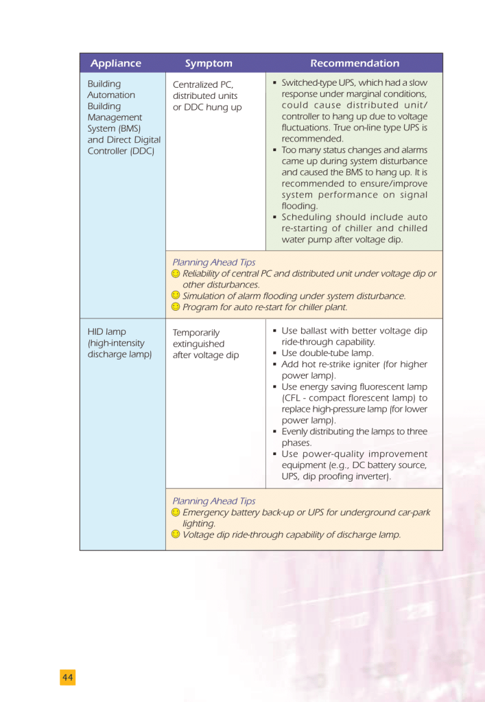
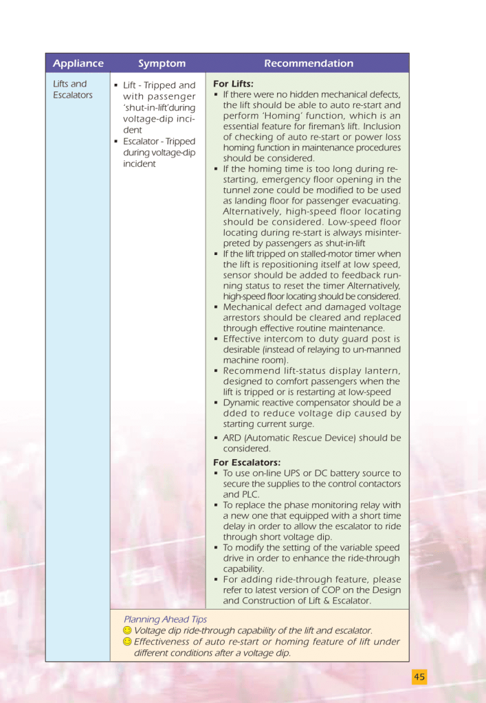
Power Quality Handbook For Your Facilities
Published by CLP, June 2007


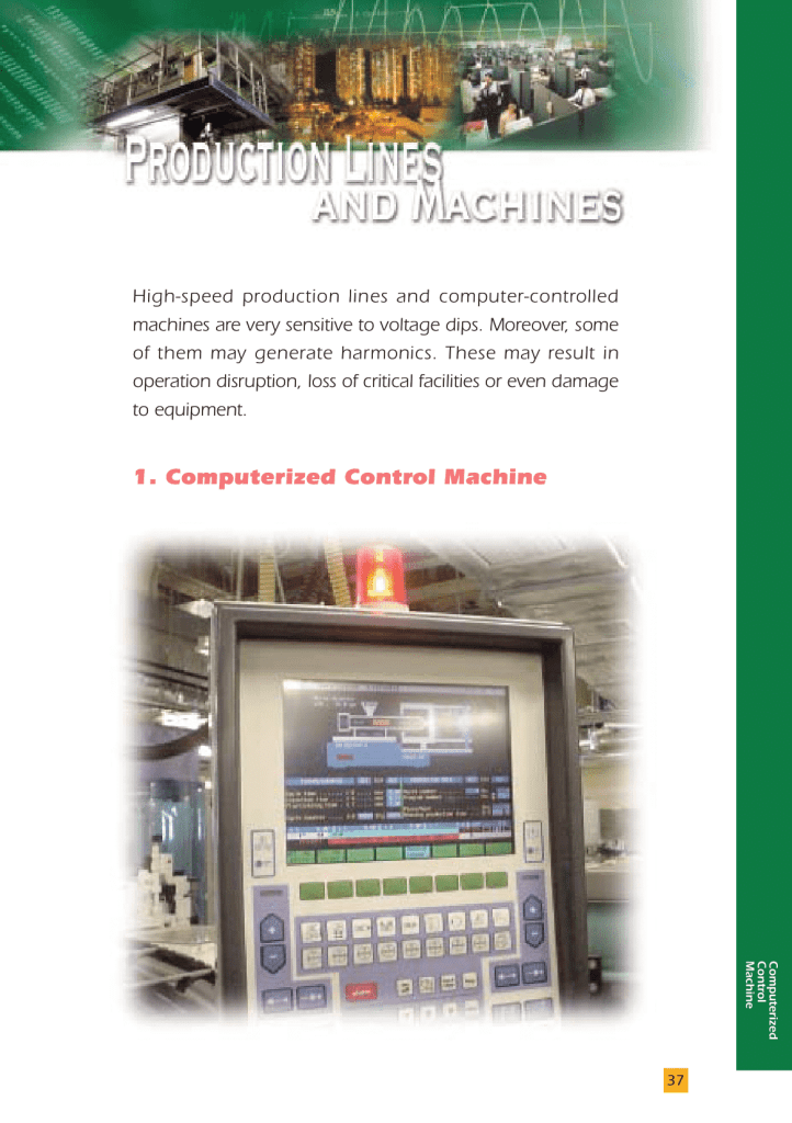


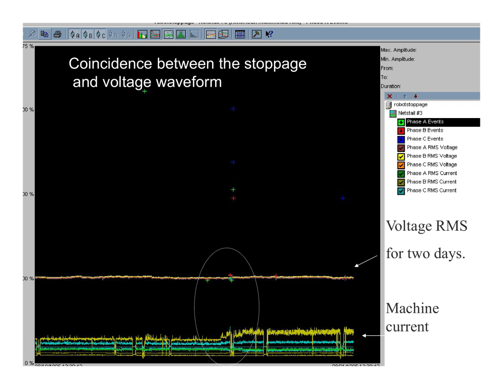
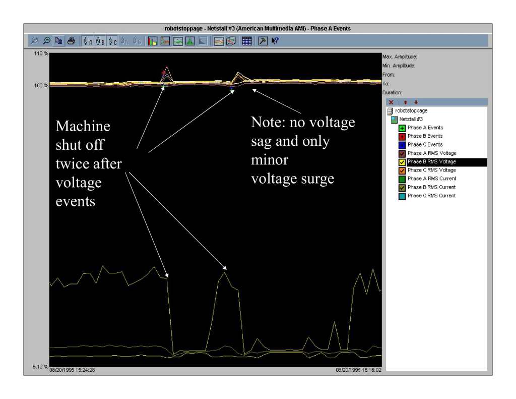
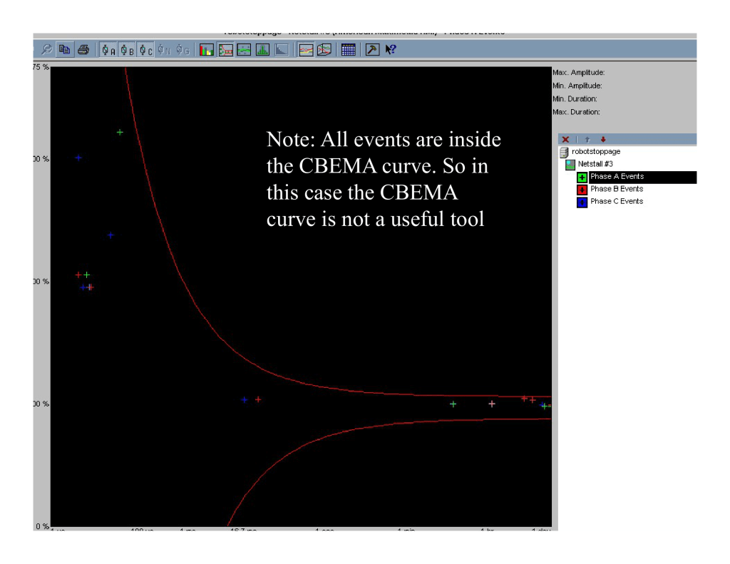
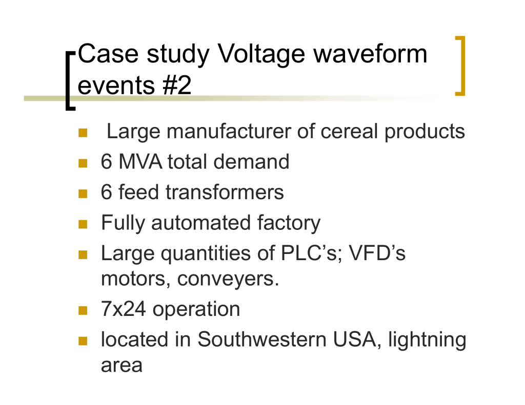
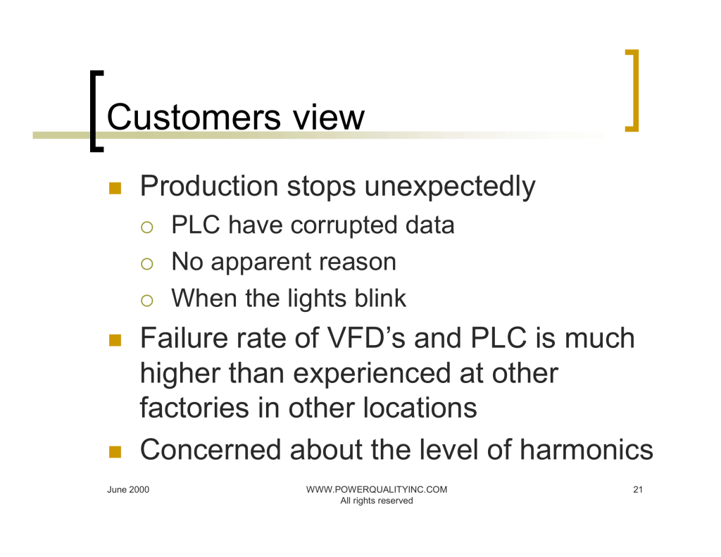
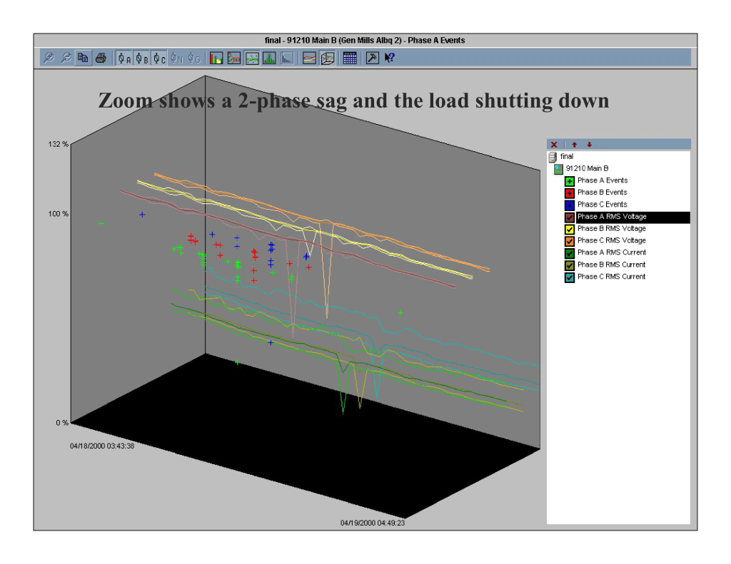
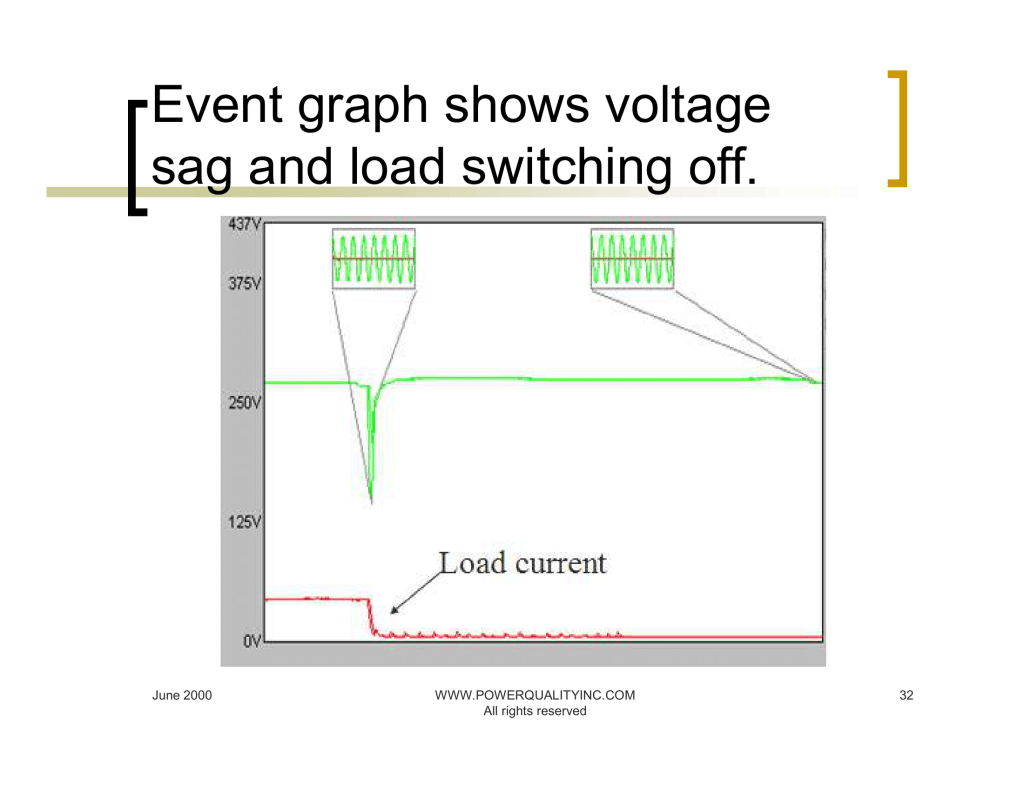
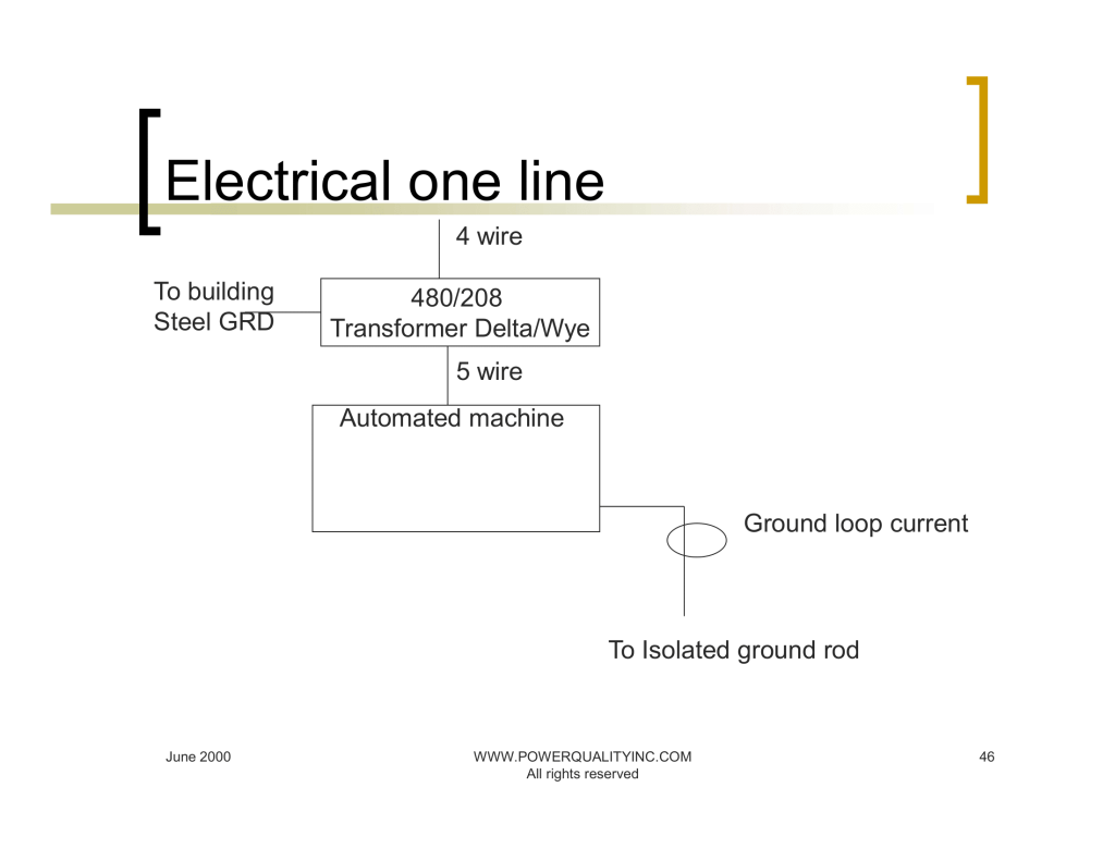
Why Automatic Machines Stop Unexpectedly
Published By Terry Chandler Director of Engineering, Power Quality Thailand LTD/Power Quality Inc., USA.
Emails: terryc@powerquality.org, terryc@powerquality.co.th
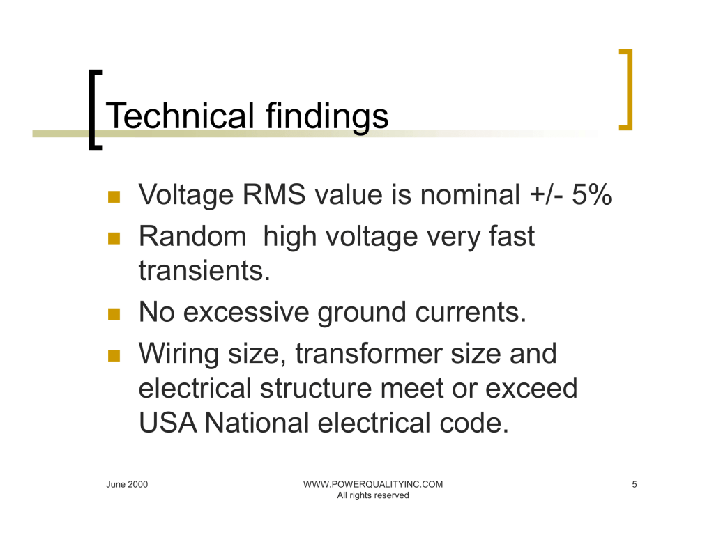
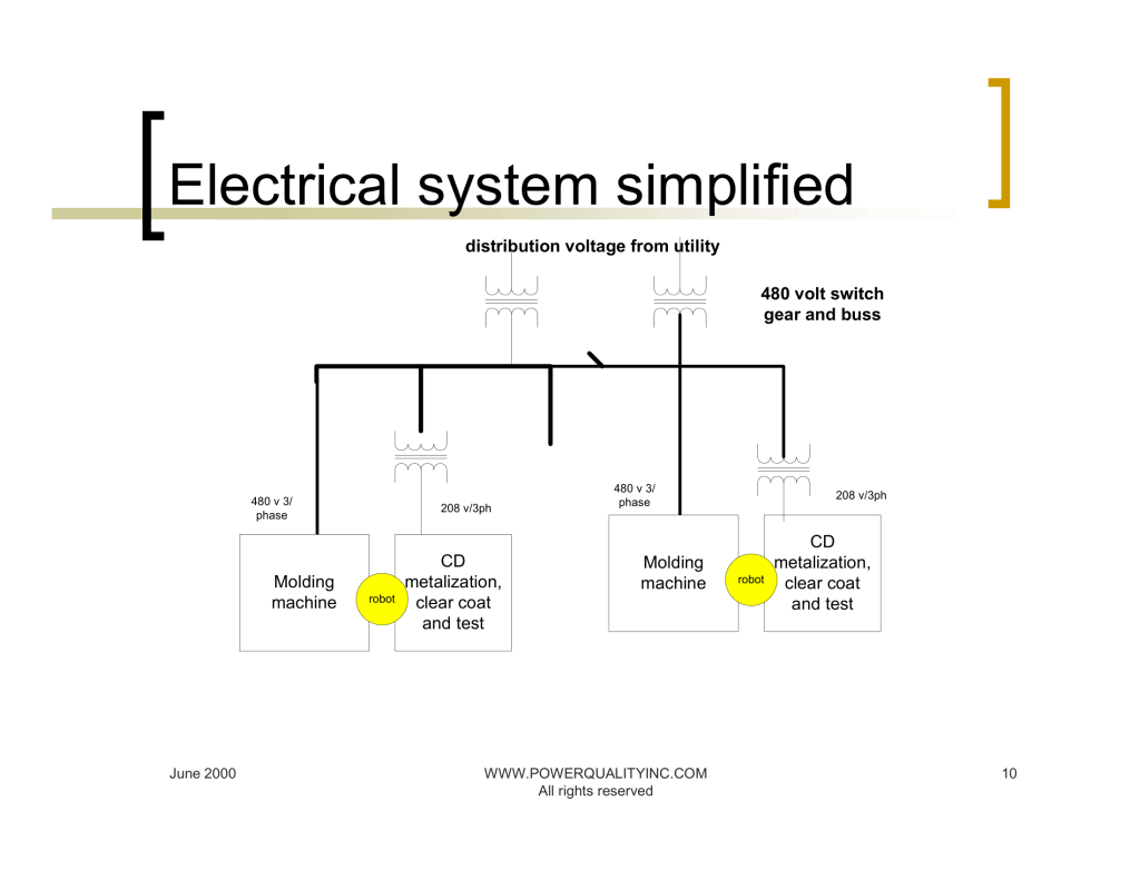
Power Quality Case Studies, June 2000


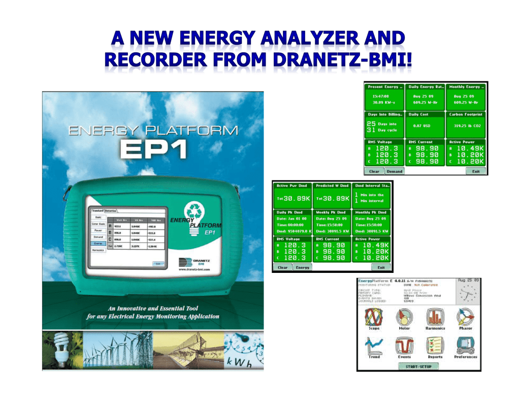
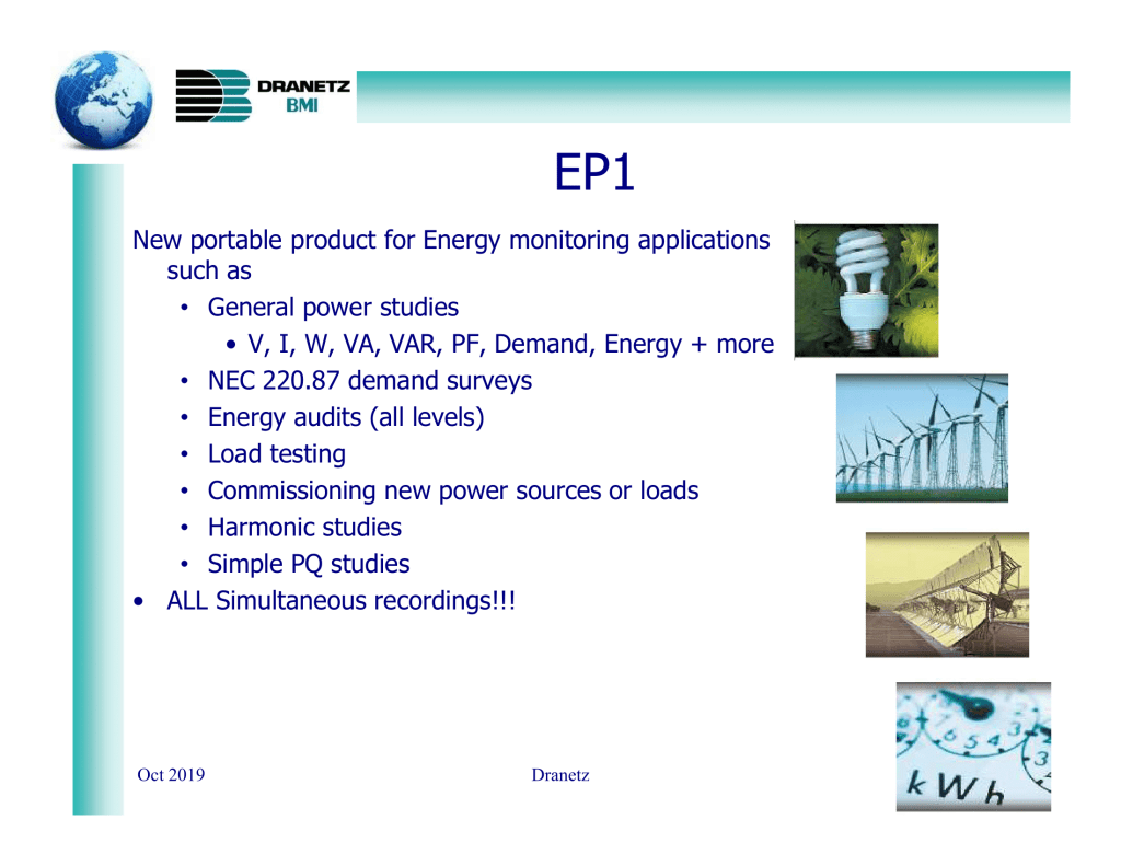
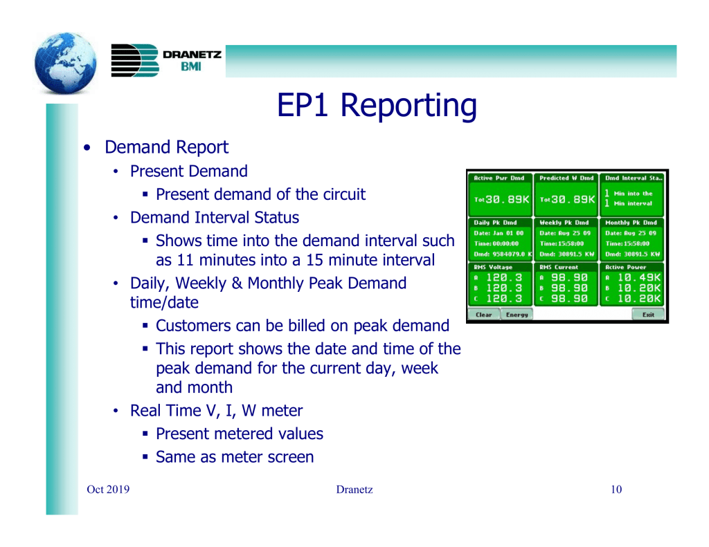
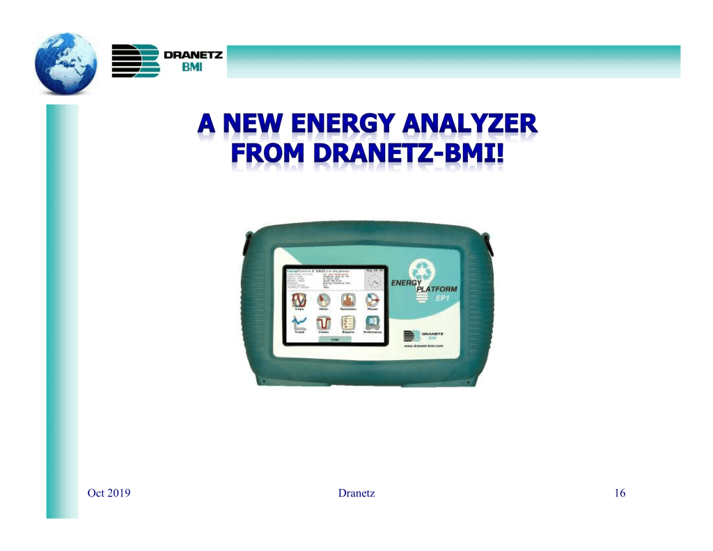
EP1 – A New Energy Analyzer & Recorder


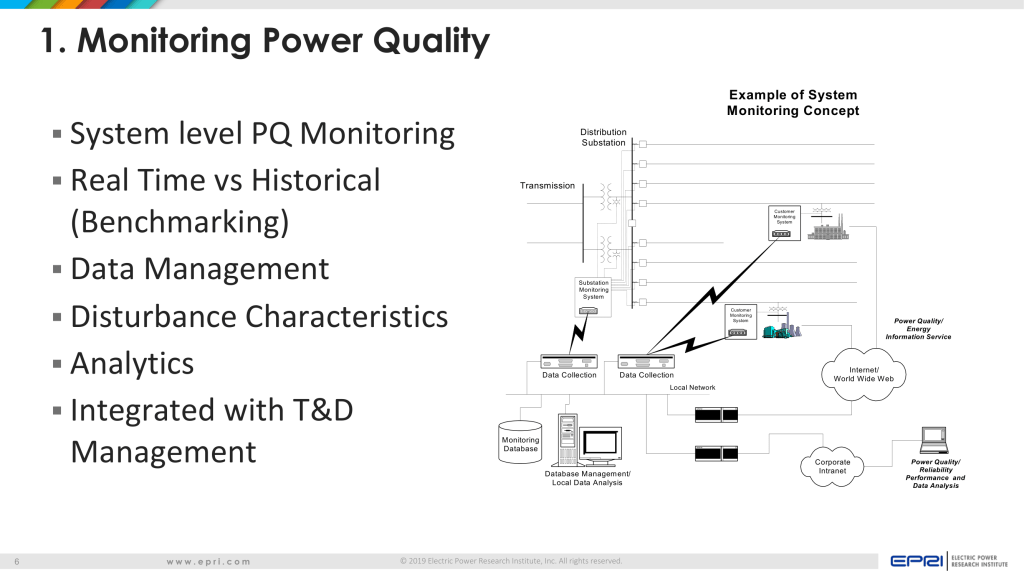
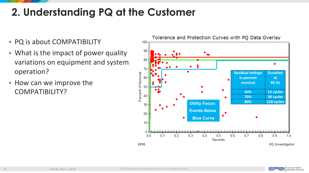
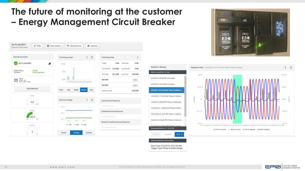
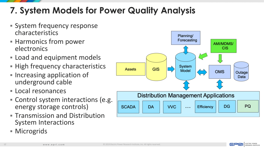
Power Quality Research Priorities
Published by Mark McGranaghan, VP, Integrated Grid, Electric Power Research Institute (EPRI), August 2020
Email: mmcgranaghan@epri.com