Published by Cypress Perform, Cypress Semiconductor Corporation, website: cypress.com
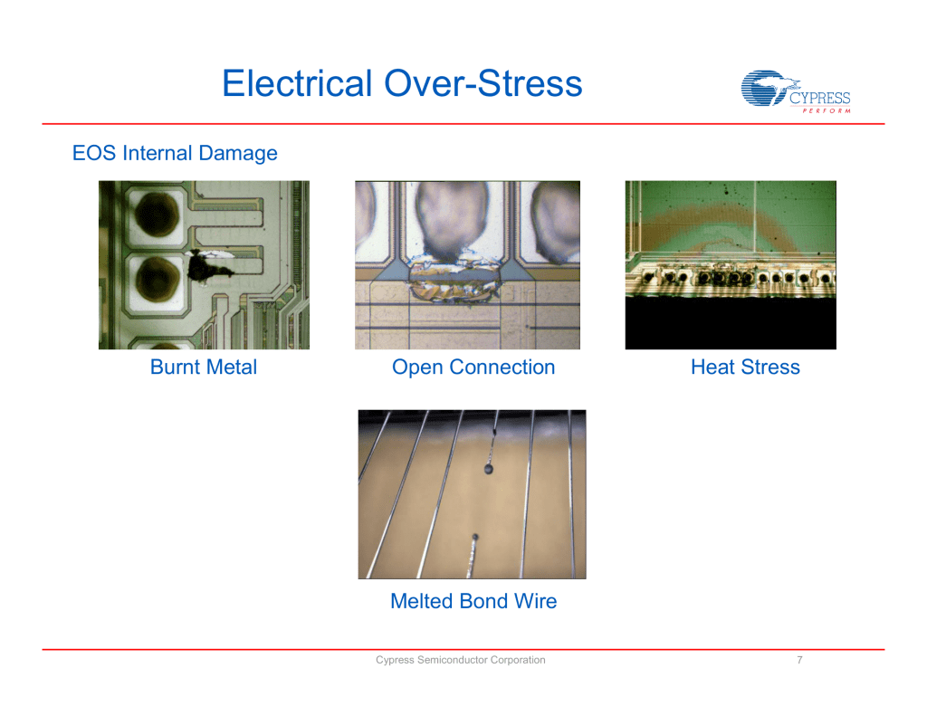
Electrical Over-Stress (EOS)
Electrical Over-Stress (EOS) is a term/acronym used to describe the thermal damage that may occur when an electronic device is subjected to a current or voltage that is beyond the specification limits of the device.
Published in PEACON & INNOVATION 2018 “PEA4.0 : Road to Digital Utility” 24th-25th September, 2018. Centra Government Complex Hotel & Convention Centre Chaeng Watthana Chaeng Watthana, Bangkok
Abstract
Nowadays the rapid evolution of power systems leads electricity system transfer from centralized fossil fuel to decentralized distributed generation (DG). The distributed generation based on single phase wind turbine generator placement and sizing problem is formulated as a nonlinear integer optimization problem. Single phase wind turbine installation in distribution systems is beneficial and requires optimal placement and sizing of this DER. However, the addition of single phase wind turbine can cause power quality problems such as over voltage levels and increasing of harmonic waveform. Hence, single phase wind turbine should be optimally located and rated taking the presence of power into account.
The goal is to minimize the overall cost of total real power losses and maintain voltage level and power quality. The optimal single-phase wind turbine placement and sizing problem is tackled by H-particle swarm optimization (HPSO). To include the presence of real power, the developed HPSO is integrated with power distribution system. The modified IEEE 13-bus three phase unbalanced radial network is used to validate effectiveness. This case study is implemented on MATLAB. The results present the necessity of including harmonics in optimal single-phase wind turbine placement and sizing to avoid any possible problems that occur with power quality issue.
In epochal years, the infrastructure of a distribution systems is extensively expanding that facing the pressure to integrate the distributed generation (DER) based such as solar rooftop PV, electric vehicle (EV), and single-phase wind generation, which are commonly penetrated in distribution systems in order to support governments policies. Consideration in the term of utility power system these penetration of DER helps reduce real power losses, release system capacity, and improve voltage profile. The achieving such benefits among other benefits depends on the most appropriate method to manage these the installation of DER, which in this paper focus on single-phase wind turbine generator.
In addition, along with voltage drops and real power loss, the growing of electricity demand requires upgrading the distribution system infrastructure, when electric loads are increasing, the voltage profile tends to decrease with the dispersion feeder being below the acceptable operating limit. The installation of distributed generation based on single-phase wind generators can help to enhance performance of utility electric power distribution systems.
However, the use of harmonic devices on the controller part of this type of DER in the widespread distribution system create the unexpected harmonic distortion throughout the system. Harmonics causes overheating due to excessive wear and and tear of electrical equipment. The integration of single-phase wind generator without considering harmonic sources in the system may lead to an increase in the total harmonic distortion because of the reflection between the control devices and the components in the system. Distorted radial distribution systems are inherently unbalance in several reason. Firstly, distribution supply both single and three phase loads through distribution transformers. Secondly, phases of transmission lines are unequally loaded. Lastly, overhead lines in distribution systems are not transposed not the same as transmission systems.
From the previous experimental the developed heuristic models, varying according to local search engine ranking of the best global single-phase wind generator, which makes the cost of losing all power to the actual performance of the DG decreases [1]. The purpose is to reduce the actual cost of power loss and the efficiency of the evaporator capacitor while observing the practical limitations. The result shows that the neglect of the presence of a harmonic source may Carpinelli et al. Correct the position of the capacitor and scale the problem in such a way that the overall cost decreases. [2].
In this paper use the same method of the problem of scaling solar rooftop PV, which is best defined as an integer programming problem is not linear, with no limitation as limitation is the rms. The voltage of the bus and the deviation of the total harmonics. One source speculated that the station utility. The heuristic algorithm, based on local variability, offers to overcome the prohibitive computational time associated with considering every potential capacitor size in a given repetition. Yan contributes to Harmonic loading in distribution systems [3].
Hybrid dynamic evolution algorithms have been developed to determine the position and the capacitance in the distorted delivery system well. Sensitivity tests were conducted prior to the optimization process to monitor the buses for reactive energy compensation. Costs related to the cost of actual power loss, spinning capacitors, and harmonic distortion. Use the estimated energy flow method and the linear harmonic flow method to calculate the cost functions at fundamental and harmonic frequencies.
Therefore, to study the effects of single-phase wind generator location and size on the increasing number of harmonic distortions, a harmonic power flow algorithm was integrated with the particle swarm optimization algorithm to calculate the harmonic related terms. These terms were the harmonic bus voltages, harmonic real power losses, and total harmonic distortions. The total real power loss and the cost of the real power loss and shunt capacitor installation were considered as objectives of the optimal DG based on single-phase wind generator locational and sizing problem.
The findings of this research indicate that the inclusion of single-phase wind generator in power distribution systems without harmonics consideration may cause a serious harmonic distortion problem, where the objective functions were subject to inequality and equality constraints. The inequality constraints were those associated with limits on bus voltages, total harmonic distortions (THD), and the total number and size of single-phase wind generator to be installed and thus, the equality constraints were the nonlinear electric power flow equations.
2. Problem Formulation
2.1 Optimal placement and sizing formulation
The main purpose of installing the capacitors in an electrical distribution system is to reduce the total power loss and also improve the voltage level in a system. The formulation of total power losses utilized in this study as the constraint parameters for the optimization solution is given in equation (1).
where, m and Nl is the feeder number and total number of feeder, respectively. In the market, the size of the single-phase wind generators is given in fixed size. In this study, a complete size of single-phase wind turbine is designed based on the combination of several generators with smallest size of rated power. Single-phase wind turbine installation cost is chosen proportional to the size of the generators. The size of the generators to be installed at the selected destination is limited to the maximum size of rated power load [4]. Where the available generator size given in Table 1. The most optimal placement and the size of the installed are referred to the cost of total power loss as expressed in equation (2).
Table 1. Available discrete single-phase wind turbine generator sizes
Model
Rated Power (kW)
Swept area sq. m
Rotor Radius
CF20
20
135
6.55
Gaia-Wind 133-11kW
11
133
6.5
CF15
15
92
5.4
Westwind 20 kW
20
82
5.2
Evoco 10
9.55
74
4.85
Aircon 10s
9.8
45
3.8
Xzeres 442SR
10
41
3.6
Bergey Excel 10
10
38
3.5
where, Ks is the cost coefficient for power losses ($/kW) and j is the number of selected buses required for the single-phase wind generators installation. The objective function from equation (2) is bounded by a number of constraints which are the allowable minimum and maximum voltage limit and limitation of generator size specified at each bus.
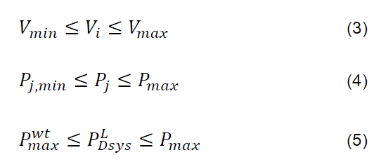
Thus, the inequality constraints considered in this study can be described as follows.
where:
Vlower bound of bus voltage limits;
Vmax upper bound of bus voltage limits;
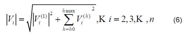
|Vi| rms value of the bus voltage and defined by
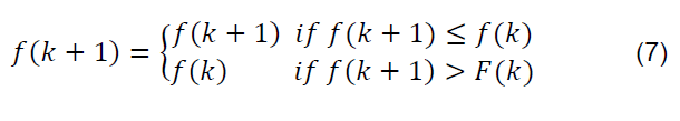
However, the minimum constraint of inductive reactive power for this study is set to zero to provide wide selection of generators sizing. The PSO technique developed for this case study will execute equations (3), (4), (5), and (6) at every computational iteration. The global best solution will not be update unless the objective function, is improved or reduced and this condition is described in equation (7).
where, k is the number of computational iteration.
2.2 Particle Swarm Optimization Technique
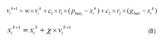
Particle Swarm Optimization was introduced by R. Eberhart and J, Kennedy, inspired by social behavior of bird flocking or fish schooling. It is a part of modern heuristic optimization algorithm, it work on population or group in which individuals called particles move to reach the optimal solution in the multidimensional search space. It works with direct real valued numbers, which eliminates the need to do binary conversion of a classical canonical genetic algorithm. The number of particles in the group is Np. The initial population of a PSO algorithm is randomly generated within the control variables bounds. Each particle adjusts its position through its present velocity, previous positions and the positions of its neighbors. Each particle updates its position based upon its own best position, global best position among particles and its previous velocity vector according to the following equations:
where:
vik+1 velocity of ith particle at (k +1)th iteration
w inertia weight of the particle
vik the velocity of ith particle at kth iteration
c1, c2 acceleration constants.
r1, r2 randomly generated number between [0, 1]
pbest i the best position of the ith particle obtained based upon its own experience
gbest global best position of the particle in the population
xik+1 position of ith particle at (k +1)th iteration
xik the position of ith particle at kth iteration
X constriction factor. It may help insure convergence. Suitable selection of inertia weight provides good balance between global and local explorations.
3. Methodology
3.1 Construction of distribution system simulation
In this study, circuitry-based commercial software has been chosen to develop IEEE 13-bus three-phase unbalanced radial distribution system. The model was designed by taking into account several important electrical components such as the three-phase load, distribution line, buses, incoming source and measurement blocks. The load flow simulation is performed which will provide the measurement in a time domain response at a steady state condition.
In Figure 1, the IEEE 13-bus three-phase unbalanced distribution system is embodied with the total real and reactive power of 3676.50 kW and 2560.90kVar, respectively. The system is considered to be unbalanced since there are several buses connected with only single or two-phase load. The sampling time of simulation is set as 50μs and 50 Hz is set for the frequency. The system is operating at the nominal voltage of 4.16 kV accept at bus 634 where the voltage is step down to 480 V.
3.2 OPF single-phase wind generator with HPS
Figure 1. IEEE 13-Bus Three Phase Unbalanced Distribution System
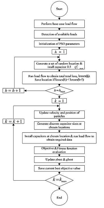
To consider harmonics, the total harmonic distortion (THD) limit at each bus is included as the optimization constraints to ensure that the harmonic distortion levels at all bus are within the allowable limits. Results of the harmonic power flow (HPF) subroutine is integrated with the PSO algorithm to determine the harmonic real power losses, and total harmonic distortions. The PSO-HPF based algorithm that incorporate HPF with HPSO algorithm show as the flow chart in Figure 2.
Figure 2.Optimal single-phase wind generator placement and sizing using HPSO technique
The procedure of PSO algorithm implemented in this study to obtain the optimal value of the objective function is discussed as follows:
Perform a three-phase unbalanced load flow solution for the original system (without the single-phase wind generator placement) to obtain the total power loss and other required data.
Start the developed PSO algorithm by generating a swarm of the particles randomly in the feasible region of the search space. As previously mentioned in section, each particle is associated with two vectors, the position vector and velocity vector.
The position vector of each particle represents a potential solution to the problem at hand. The feasible swarm is passed to the RDPF subroutine as initial guess to minimize power mismatch equations.
Each particle recalls its best position associated with the best fitness value (e.g. the real power loss). Each particle records the best position achieved by the entire swarm.
Update process of particles’ positions results in continuous values of particles’ positions and made discretization of particles’ position vectors.
Feasible check the particles to ensure that no particle flies outside the feasible region.
4. Results and Discussion
The algorithm of PSO technique and a case study of IEEE 13 bus three-phase unbalanced distribution model were developed in MATLAB. The HPSO is executed for 10 times with 100 iterations of optimization process is specified for each time.
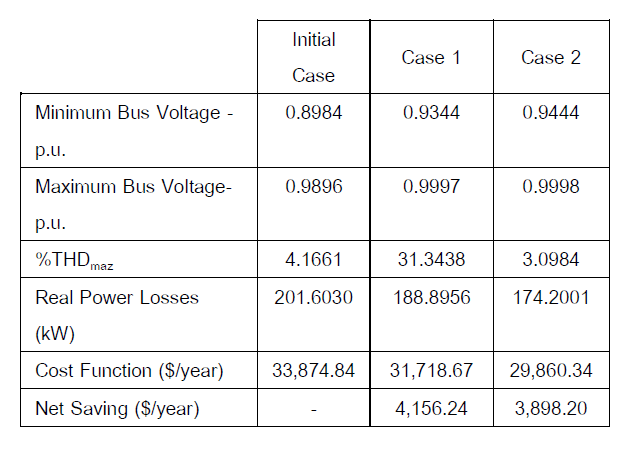
With the presence of harmonics, two different cases investigate the impact of single-phase wind generators installation on the voltage profiles, total harmonic distortions, total real power losses, and total cost are considered.
Case 1 represents the system without total harmonics consideration after single-phase generator installation.
Case 2 represents the system with harmonics consideration after single-phase generator installation.
Table 2. Available discrete single-phase wind turbine generator sizes
The maximum number of iterations was taken as 100 for the tuning process of each parameter. It was found that the PSO algorithm was less sensitive to its parameters when the problem dimension was small (the problem dimension was single-phase wind generators). However, the larger the problem dimension is, the more sensitive the PSO algorithm becomes. The solution of the optimal solar rooftop PV placement and sizing problem using developed PSObased algorithm was able to find optimal locations and that overall cost was minimized. The simulation results for initial case, cases 1, and 2 is reported in Table I. Based on Tables II execution gives the best solution with respect to the best total cost considered as its objective function.
The convergence characteristics of the developed PSO-HPF-based approach for cases 1 and 2 in the optimal placement and sizing of solar rooftop PV problem with the total cost being the objective with HPSO consideration is depicted in Figure 3.
Figure 3.
4. Conclusion
In this paper, the single-phase wind generator placement and sizing problem was formulated as a constrained nonlinear integer programming problem with both locations and ratings of single-phase wind generator is discrete. The constraints considered were of two types: equality and inequality. The equality constraints were the nonlinear power flow equations. The developed PSO-HPF-based algorithm was tested on an unbalanced 13-bus test system to calculate the optimal locations and sizes of single-phase wind generator taking harmonics into account.
Reference
[1] Y. Baghzouz and S. Ertem, “Shunt capacitor sizing for radial distribution feeders with distorted substation voltages,” IEEE Trans. Power Del., vol. 5, pp. 650–657, Apr. 1990. [2] “Systems with harmonic distortion,” in Proc. IASTED Int. Conf. Power and Energy Systems, May 13–15, 2002, pp. 352-353. [3] G. Carpinelli, P. Varilone,“Capacitor placement in three-phase distribution systems with nonlinear and unbalanced loads,” Proc. Inst. Elect. Eng., Gen., Transm. Distrib., vol. 152, pp.47–52, 2005. [4] A. Eajal, S. Member, and L. Fellow, “Unbalanced Distribution Systems with Harmonics considered Using PSO,” vol. 25, pp. 1734–1741, 2010. [5] P. Sudta “Optimal DG Based on Solar Rooftop PV Placement and Sizing in Unbalanced Distribution Systems with Harmonics Consider Using PSO” PEACON2017
Mr.Chitchai Srithapon, Customer Service Division, Provincial Electricity Authority, Email: chichai.sri@pea.co.th
Mr.Pichai Thaniwan, Customer Service Division, Provincial Electricity Authority, Email: phichi.tha08@gmail.com
Mr.Weerachat Khuleedee, Customer Service Division, Provincial Electricity Authority, Email: weerachat_ee35@hotmail.com
Mr.Wacharapong Rakapong, Information System Division, Provincial Electricity Authority, Email: nidpea@gmail.com
Published in PEACON & INNOVATION 2018 “PEA4.0 : Road to Digital Utility” 24th– 25th September, 2018. Centra Government Complex Hotel & Convention Centre Chaeng Watthana Chaeng Watthana, Bangkok
Abstract
According to the service standard policy by the Energy Regulatory Commission (ERC) of Thailand in 2016, made all of electricity utilities have to verify meter accuracy of all residential customer meter to make sure all meters measure reading is precision in accuracy class of 2.5% for every 3 years. Today, Provincial Electricity Authority (PEA) has the existing residential customer kWh meters about 17 million, where it required many work task and high budgets to achieve this mission. Therefore, PEA team had developed the on field meter accuracy testing system to be able to perform operating faster and make a cost saving.
The proposed smart system was designed to complete with a new meter tester feature and new software implementation on both internet web service and smart phone application. The implementation of this mobile workforce has showed that the meter accuracy investigation in field site capacity per day increased by 67.6% and could save testing investigation cost about 38.9% when compare with the traditional method.
Key words: Innovative, kWh meter accuracy, mobile workforce.
1.Introduction
Currently, the electrical industry structure in Thailand is the enhanced single buyer model, the Electricity Generating Authority of Thailand (EGAT) is a producer of electricity for power transmission and is the sole purchaser of electricity from private power plants and buys electricity from abroad, then will distribute electricity through the transmission system to the Provincial Electricity Authority (PEA) and Metropolitan Electricity Authority (MEA). By the Energy Regulatory Commission (ERC) of Thailand is responsible for overseeing the overall electricity tariff structure.
PEA who is the biggest power utility in Thailand, supervise power distribution and electricity energy retail system for most provinces areas of Thailand, except only for Bangkok metropolis, Nonthaburi and Samutprakarn province that responsible by the MEA. PEA is the state owned enterprise of Thailand, which is the owners of the power transmission lines, power substation, distribution system, mini hydro power plant and kWh meters. The description of PEA importance data is show in Table 1.
Table 1. PEA Importance data [1]
Description
Data
Power line (circuit-km)
H.V. Transmission Line
12,258
M.V. Distribution Line
308,958
L.V. Distribution Line
462,786
Number of power substation
544
Number of Customers
19.35 million
Total Sales of Electricity (kWh)
132,399 million
Total Assets (Baht)
398,305 million
Year revenue (Baht)
463,747 million
According to the service standard policy by the Energy Regulatory Commission (ERC) of Thailand in 2016 [2], made all of electricity utilities have to verify accuracy of all residential customer meters to make sure its reading accuracy is in class 2.5% for every 3 years. Today, PEA has the existing residential customer meters about 17 million meters and most of them are electromechanical meter type. The number of new meter in first 3 years installing that was verified accuracy by factory test has about 3 million and the installed meter with more 15 years old that will be planned to replace by new meter has about 2 million per year. That means the number of meter that PEA have to verify meter accuracy under ERC policy about 4 million meters per year. The operation cost of meter accuracy testing separate by operating method is shown in Table 2. The operation cost of meter accuracy testing in laboratory is about 540 million THB per year and for on field meter testing about 240 million THB per year. Therefore, it is reasonable to do meter accuracy testing job in the field site.
Table 2. Operation cost of meter accuracy testing by method
Method
Laboratory Test
On Field Test
Number of meters testing per year
4,000,000
4,000,000
Testing cost/meter
135 THB
60 THB
Total cost/year
540 million THB
240 million THB
In this paper, we first describe the on-field meter accuracy testing methodology in Section 2. In Section 3, the new system implementation result is presented. In Section 4, the paper is briefly concluded.
2. On-Field Meter Accuracy Testing Methodology
The traditional methodology of on field meter accuracy investigating for residential customer meter in PEA is worked with a standard clamp on meter and testing results was recorded in hard paper form [3],[4]. In the case of a customer kWh meter no load current that mean no any energy reading in that time, to can do a meter accuracy testing it need to unplug the power cord in customer load side and reconnect with the dummy load such as a light bulb or a heater coil. That it made this method has a long time for meter testing and may interrupt electricity usage of customer. The working capacity for on field meter testing by the traditional method is about 30 meter per day, where it was required many technician staff and high budgets to achieve this mission. Therefore, PEA team has proposed the new system for on field meter accuracy investigation that can be able to perform operating faster and benefit to the operation cost saving.
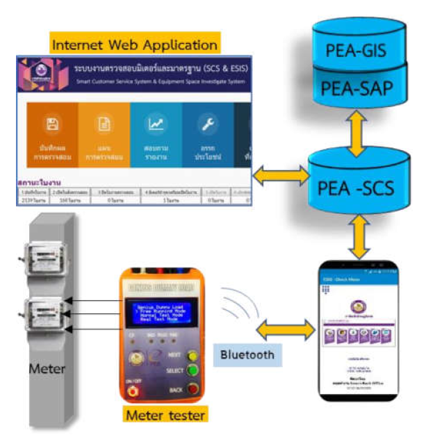
The smart on-field meter accuracy investigation system was developed to be able perform faster on field meter testing and to keep the testing results in to digital file (paperless), that could be saved much more operation cost in this work. This smart system is designed to complete with an innovative meter tester and the new software applications on both internet webpage service and the smart mobile phone application. The diagram of the smart on field meter accuracy investigating system for PEA 4.0 is shown in Figure 1.
Figure 1. The diagram of smart on field meter accuracy investigation system for PEA 4.0
2.1. The Innovative Meter Tester
This innovative meter tester is named as “GDL”, it was designed for 1P2W meter testing. It was completed with an internal current source, to make the kWh meter reading (rotating) in case of no customer demand current. This smart meter tester was calibrated with standard meter tester (accuracy class 0.1%) at instrument calibration laboratoy in Meter division, PEA and had passed accuracy qualification in class 0.5%. GDL also was built in the Bluetooth communication module to sent the testing result to a smart mobile phone. This smart tester also can be used to measure the electricity consumption parameters such as voltage, load current and demand power in during meter testing. After completed testing, it will be displayed the testing result on its LCD display monitor and sent the testing data to a smart mobile phone or smart mobile tablet. The system diagram of GDL is shown in Figure 2.
Figure 2. The system diagram of GDL
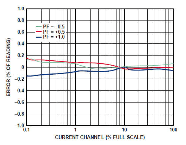
The meter tester will measure the voltage and currents waveform from kWh meter under testing through the ADE7953 IC chip [5]. This IC chip is use to measure power and energy parameter and the example of active energy error reading as a percentage by this IC chip is shown in Figure 3. The accuracy testing by this method is to compare the energy measurement between the GDL reading and a kWh meter reading in the same period testing.
Figure 3. Current Channel B Active Energy Error as a Percentage of Reading (Temperature = 25°C) over Power Factor with Internal Reference, Integrator On
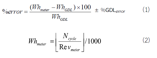
The error as a percentage calculation of a kWh meter accuracy testing is derived by equation (1) and (2).
Where:
% error is the accuracy of kWh meter under tested.
Whmeter is energy (Watt-hour) reading from meter.
WhGDL is energy (Watt-hour) measure by GDL tester.
GDLerror is %error offset of GDL form calibration laboratory.
Ncycle is the number of testing cycle.
Revmeter is constant value of kWh meter reading.
2.2. Software Applications Development
This smart system is operated via online system with software applications that used to interface with the PEA smart customer service system (SCS). The software applications were developed on both internet webpage service and smart mobile phone application. The webpage application use for on field kWh meter testing in job planning, generate working order, testing result recording and test data reporting.
The example of internet webpage application is shown in Figure 4.
Figure 4. The example of webpage application for on field meter investigating system
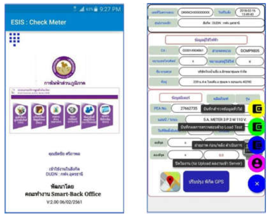
The mobile application was design to use in field site that can be download meter information from the PEA-SCS system such as customer name, supplier and installation date etc. A smart phone can be communicated with GDL by Bluetooth signal to receive the test result and then record data in mobile memory. Ones it has internet signal maybe from Wi-Fi system or GSM signal, it will can be uploaded the testing data into database server. This application also has the meter locator finding function by interface with the data from PEA Geographical Information System (PEA-GIS) where keep the x-y location of the customer meter and can be sent back the current meter location into the GIS database. The example of mobile application for this smart on field meter accuracy investigating system is shown in Figure 5.
Figure 5. The example of mobile application for the smart on field meter investigation system
3. System Implementation
The smart on-field meter accuracy investigation system has deployed in Northeastern regional of PEA since August 2017. The example of system implementation in the field site is shown in Figure 6.
Figure 6. The example of new system implementation in field site
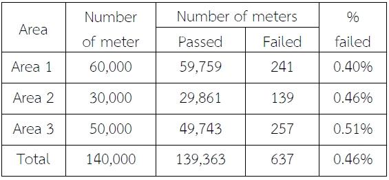
The data of meter accuracy testing result by 4 months system implemented with 140,000 meters sample data is shown in Table 3. The result is shown the new innovative meter tester can be detected the failed kWh meter that reading accuracy out of class 2.5% in distribution network. By the failures rate is about 0.46% which those failed meter were confirmed testing in PEA meter testing laboratory with a same result.
Table 3. On field meter accuracy investigating data
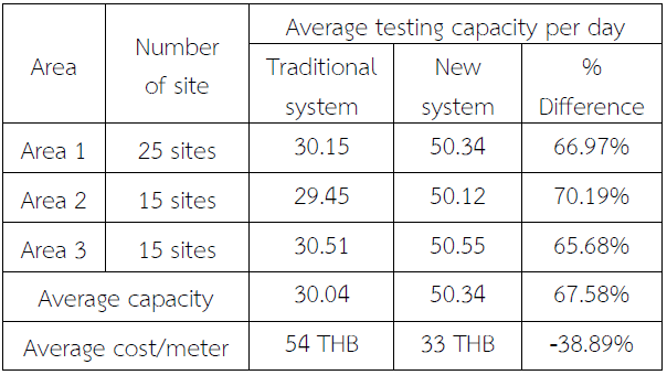
The result of working performance based on number of on field meter testing capacity per day is shown in Table 4. Data shows the new smart system for on field meter accuracy investigating can be tested accuracy about 50 meters per day, while in the traditional system can be done about 30 meters per day. That means this new smart system developing can be performed operating performance improvement about 67.6% when compare with the traditional system.
Table 4. On field meter testing capacity
For the operation cost comparison between the new propose system and the traditional system is shown the operation cost by new system is lower than the traditional method about 38.9%. Where it can be saved the PEA operation cost budgets for on field meter accuracy testing for 4 million meters in yearly target about 210 million THB.
4. Conclusion
This mobile workforce system for on field meter accuracy investigating in PEA, that consist of the innovative meter tester and the new software applications on both internet webpage service and a smart phone application. The innovative meter tester was designed for 1P2W meter testing, which completed with an internal current source for testing a kWh meter in case of no customer load current. The new software application is used for job planning, working order generated and testing reporting. The developed smart phone application can be communicated with the meter tester by Bluetooth signal to receive the testing result. And then it will be uploaded the testing data to the PEA database server by internet protocol.
The new system implementation has been shown the on field meter accuracy testing working efficiency improvement, by increase the on field meter testing capacity per day about 67.6% and can be saved the operation cost about 38.9% when compare with the traditional methodology. The other advantages of this new smart system is benefited for distribution system improvement such as the voltage from meter testing can be used to monitor voltage quality in network area. The mobile phone position (x-y) in a same position of tested meter will be used to correct a meter location in PEA’s Geography Information System (PEA-GIS) and the meter accuracy testing data also keep in digital database server that it is very useful for another data analytic application in the future.
Acknowledgment
The author would like to thank the support team for this project implementation in Northeastern regional. And this the innovative meter tester development was supported by Provincial Electricity Authority innovative funds in 2017.
References
[1] Provincial Electricity Authority (PEA), “PEA Annual report 2017”, Bangkok, Thailand, 2018, [2] Energy Regulatory Commission (ERC), Thailand, “Power Purchase Agreement (Small power users) in accordance with the standard of electrical service contracts, 2017”, pages 11-13., 2017. [3] Provincial Electricity Authority (PEA), “PEA Regulations on Meter Metrology Practices,” pages 89-90, 2015. [4] Provincial Electricity Authority (PEA), “Electrical Equipment Specification No: RTES-136/2539, a class 0.5 standardized meter, is available for single phase test “, page 4, 1996. [5] ANALOG DEVICE, “ADE7953 Data Sheet,” MA, USA, 2011.
Our instruments are great, but Dran-View 7 software makes them better! Much more than just a viewer, Dran-View adds value to any power survey. Used by tens of thousands of power professionals, Dran-View is included with most of our portable instrument packages, including HDPQand DranXperT:
Want to see and hear more about Dran-View 7? Our Webcastpage now has 13 Dran-View training videos covering basic, intermediate and advanced topics. Learn everything ranging from the basics of opening files, viewing data and navigation to advanced topics such as harmonic computations and creating your own math channels.
Published by Dr. Sioe T. Mak, Power Quality Specialist and Steven E. Spencer , President – CEO, ADVANTAGE ENGINEERING, Inc.
769 Spirit of St. Louis Blvd., Chesterfield, MO. 63005, USA, Tel. 314-530-0470, Fax. 314-530-0670, E-mail ae@inlink.com
ABSTRACT
Many small and medium size industries and very large farming operations move into rural areas and small towns equipped with the latest technologies in motor drives, power electronics for process control, welding apparatus, etc. They generate non-linear loads and create unique power quality problems. The fairly low capacity medium voltage substations serving these loads also aggravate these problems. Numerous complaints about light flicker, poor voltages, early equipment failures are on the rise and in many instances it requires good electric detective work to determine the source or main culprit of the power quality problem.
A data acquisition tool with specially designed multifunctional application software was successfully used by the authors in the field investigation to identify the causes of the problems mentioned above. A brief description of the functional capabilities of the data acquisition unit will be presented.
Some important case studies and a listing of commonly encountered problems will also be presented in the paper. Some hidden problems will also be identified. Suggestions to improve existing power quality standards, definitions of tolerable limits, test laboratories, etc. will also be discussed.
GENERAL INTRODUCTION AND ASSESSMENT OF POWER QUALITY ISSUES
Several years of investigative work at hundreds of sites at many electric utilities reveal a multitude of problems, which can be classified as power quality problems. They can be broadly divided into several categories.
Problems generated by the electric utility causing problems at the customers’ premises.
Problems generated by a customer causing problems to other customers.
Problems generated by a customer causing problems to his own equipment.
On the electric utility side many of the problems seemed to be related to voltage regulation, capacitor banks placements and sizings, line design, transformer sizings, etc. The electric utility is assumed to generate 60 Hz power with some uneven harmonic components due to transformer magnetizing currents only.
At the customer’s side most of the problems are generated by electric welders, rectifiers and variable speed drives, switching power supplies, motors and motor starters, broken or poorly connected equipment, heavy unbalance loading, inadequately designed low voltage network, etc.
The natures of the problems are voltage distortions, transients, voltage sag or swell and voltage unbalance. On many occasions customers blame the utility or another customer for the cause of their problems.
During the past 15 years, a dramatic increase in problems caused by high harmonics was observed and seems to be worsening as time goes on. Thus far we only see the tip of the iceberg.
In the newly deregulated environment, the mandatory requirement to serve a load to a customer inside the utilities’ service territory is slowly disappearing. Instead, the retail wheeling concept allows utilities and customers to sell and buy power based on competitive pricing like any other commodities.
Utilities are also thinking of imposing limits of voltage distortions that customers’ loads generate. The customer will be responsible for improving their load power factor. In order to survive, electric utilities have to improve customer services. If at one time the utilities served the role of reliable power provider only, new types of appliances and equipment generating new types of electric phenomena literally force the utility to expand customer services into areas that they are not too comfortable with. Also unique for the smaller utilities serving smaller towns and rural areas is the explosive growth of small to medium size industries and commercial institutions in their service territories. To meet the increased demand it is necessary to upgrade the distribution network.
To avoid finger pointing when a problem arises, it is necessary to identify the source and the cause of the problem and who is suffering from the problem. This requires a certain degree of expertise and the availability of monitoring and analytical tools that are easy to operate. Upgrading of substations, the distribution network and operating tools are unavoidable and costly. This burden has to be shared with the customers. Will the customer accept this without improvements in services?
There is also a strong need for more comprehensive standards for power quality that utility engineers can utilize directly. Harmonic pollution limits have to be defined which can be used to implement operating policies such as penalizing the customer that generates the pollution, sharing the costs of installation upgrades, consulting, etc.
TYPICAL POWER QUALITY PROBLEMS AND CASE STUDIES
Several cases of power quality problems are listed below and some detailed case studies are also presented in later chapters. These actual cases illustrate the confusions and misconceptions that typically occurred when customers experienced problems.
A cookie baking company has microprocessor based process control equipment that kept aborting its operation. The initial suspicion was that the utilities’ feeder conductors and transformer size are not adequate to handle the load and leading to occasional short-term voltage sags. A more in depth investigation showed something different. The transmission substation that belongs to the investor owned utility from which the smaller utility buys power, had many instantaneous circuit breaker trippings and reclosings. During a period of one month 11 of such operations were detected. The solution was to switch the feeder to another source.
At a cooperative farm maintenance office building the complaint was that once the fluorescent lights go out it is very difficult to restart the lights again. The first thought in peoples’ minds was that there was a power quality problem. It turned out that the old fluorescent lights had been replaced by new quick start ones. But the old style ballast was not replaced.
At a manufacturing plant voltage unbalance was observed. The distribution transformer tap setting was low and to boost the low voltage, a three-phase autotransformer was used. One phase was used to supply power to the adjacent main office. The load at the office was large enough to cause unbalance at the plant. Because of the unbalance, motor starting times were longer causing visible nuisance light flickers.
A new motel repeatedly experienced damage to the window cooling and heating units of the individual rooms. The story we received seemed to give the impression that many of the window units were destroyed. The electric utility was blamed for the cause of the problems by not providing overvoltage protection. A careful investigation revealed that the extent of the damage was only at the electronic control board. The electronic circuitry does not have any surge protection. Each time the window unit was repaired, the same type of electronic control board was used for replacement. Hence the same type of problems keep on recurring.
These few examples clearly show that in some cases what is perceived as a power quality problem may have nothing to do with power quality supplied by the utility. Yet it is also necessary to perform a field investigation to determine the cause of the problem and thereby eliminate finger pointing.
This leads to the subject of instrumentation for measurement and monitoring [3]. Most data acquisition units available in the market are expensive and in many cases highly specialized in terms of their functionality and quite often require a high degree of expertise to operate. In order to do site investigation, the data acquisition should be easy to operate and without too much typing of specific commands or looking into multilevel menus. It should be capable to do a quick assessment about the quality of power. The ability to do long-term monitoring is also necessary. Also, anyone should be able to use a set of simple instructions to collect specific data that lends itself for detailed analysis by an expert. The device has to be a multi-channel voltage and current measuring unit, a device for very short-term and long-term monitoring and also capable to take large amounts of raw data for detailed analysis. Supporting software tools, easily expandable and flexible for on site analysis and report generation should be an integral part of the device. Advantage Engineering practically has to design its own unique data acquisition unit to facilitate the field investigation that covers a very broad range of types of problems.
The next chapter presents several interesting field studies in greater details.
CASE STUDIES
A Case of Tree Trimming
A medium power television station recently suffered occasional outages. The engineer in charge of the television station blamed a farm equipment repair shop as the main culprit of the outages. This repair shop is fed from the same medium voltage feeder as the television station and is located about one mile away from the station. After our investigation, the following was found:
A single-phase undervoltage relay at the television station was connected to phase VAN only.
An interview with the television engineer revealed that the undervoltage relay tripped during periods of high winds preceding a thunderstorm.
The outage periods had no correlation with the working hours of the repair shop.
Studying the voltage waveform and its harmonic content at the electric service entrance point of the repair shop revealed nothing unusual that can cause power quality problems.
After patrolling the feeder it was found that phase VAN was very close to the branches of several poplar trees. A wind gust can easily cause the branches to whiplash and touch the feeder conductor of phase VAN. The solution was for the utility to do tree trimming. It was recommended to increase the undervoltage relay time delay by a small amount.
A Case of Voltage Distortion, Swell and Sag
The medium voltage network of a small town is served by a 34.5 kV subtransmission line. During working day hours, fluorescent lights flickered, speed variations of cooling fans of computers and electronic devices emitted very low frequency audio noises, some uninterrupting power supplies for banks of computers switched in and out, etc.
A harmonic analysis performed on the voltage waveforms at different locations in town revealed a slight increase of the 5th harmonic compared to what one normally observed. The Total Harmonic Distortion was well below the norm of 2.5% [1]. The RMS voltage monitoring device did not indicate swell or sag of the voltage beyond the normally tolerated range. The first assessment of the situation was that somewhere in the network, a sequence of short duration nonlinear loads might be the culprit.
A data acquisition unit was used to collect voltage data at a sampling rate of 25 kHz at the moment when light flicker was observed. To extract burst type phenomena from the voltage waveform a type of comb filter was applied to the voltage sampled data. The filter equation is as follows:
Equation (1):
R ( j ) = S ( j ) – S ( j + mN )
S ( j ) is the jth sample point of the voltage. S ( j + mN ) is the (j + mN)th sample point of the voltage. M is an integer. N is the equivalent of a period of the fundamental of the voltage waveform. R ( j ) is the residue
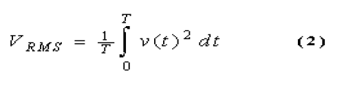
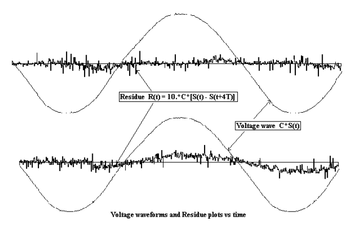
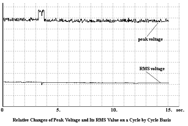
The residue obtained by choosing m = 4 by sweeping the values of j between 1 and a few hundred thousands were quite revealing. Sampled set of values for the residue in relation to the voltage waveform is shown in Figure 1. The comb filter filters out the steady state fundamental harmonic and all its integer multiples and the dc component of the voltage. A short duration swell of the voltage and all kinds of transient spikes are visible on the lower waveform in Figure 1. The upper waveform shows some non-integer harmonics and transient spikes. A plot of the variations of the RMS voltage on a cycle by cycle basis using equation (2) and simultaneously plotting the peak voltage using the same time scale is shown in Figure 2.
Figure 1: Voltage waveforms and Residue plot vs time
While the peak values vary quite a bit, the RMS values of the voltage seem to be constant. A hump visible on the peak value plot lasted close to 0.75 seconds. The short transients are caused by an interruption of arcs. The noninteger harmonics are in general transient oscillations and is a network response to load discontinuities. It was also observed that sag and swell of the voltage occurred lasting for a few cycles only. This type of phenomena indicated that a limited short circuit has occurred.
Figure 2: Relative changes of Peak Voltage and its RMS value on a cycle by cycle basis
Taking all this combination of observed phenomena, the type of load had to have a lot of arcing followed by limited short-circuits. The conclusion was that an electric welding plant generated all the perturbations on the voltage waveform.
Later verifications indeed proved that it was a medium size manufacturing plant that operated a number of large electric welding equipment. This plant was served directly by the 34.5 kV subtransmission that also provided power to the small town.
A Case of Unbalanced Voltages
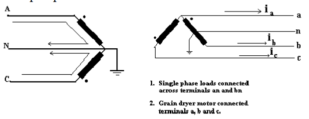
To save on conductors, some branches of the medium voltage distribution circuits use only two phase wires and a neutral. Figure 3 shows the step-down transformer to the service level voltage. It uses an Open Y – Open Delta configuration. One of the Open Delta windings has a grounded center tap connected to a grounded neutral wire. The line to line voltage has a nominal voltage of 240 V and the line to neutral voltages are 120 V and is primarily intended for light single-phase loads. This particular configuration is adequate for serving moderate size farming operations where 3 phase motors are used for blowers and small pumps.
Figure 3: Open-Wye Connection
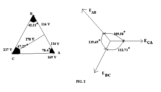
The situation that was encountered occurred at a farm that throughout the years has grown from a relatively small operation into a fair size farming business. The repeated complaint was that some of the fairly large grain drying blower motors kept tripping the breaker after starting. An electrician decided to change the setting of the thermal trip delay by increasing it an additional 20 Amps. The time delay before the breaker tripped was indeed increased but it did not really solve the problem. A conducted field investigation revealed that fairly large single phase heating loads are connected to the 120 V sources and causes large voltage drops in one of the transformer windings. Voltage measurements showed that VAB = 232 V, VBC = 237 V and VCA= 169 V. The phasor diagram is depicted below in Figure 4.
Figure 4: Unbalance Phasor Diagram
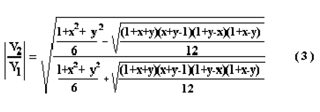
The degree of unbalance can be calculated using the following formula (3) where x = VAB/VCA and y = VBC/VCA. By inserting the values of the measured line to line voltages into the equation, the ratio of the negative sequence voltage with respect to the positive sequence voltage is found to be equal to about 20 % [7]. This unbalance generates negative sequence fields rotating at twice the positive sequence rotational speed in the opposite direction. It not only creates negative torques, which increases the slip, but it also generates additional motor heating of the iron. Because of the increase of slip, the induction motor operating current increases and this may be the cause of thermal tripping of the motor breaker.
The obvious solution is to balance the voltages by balancing the loads and to meet the required demand; the 2 phase medium voltage branch circuit has to be upgraded to a 3 phase branch circuit. At the same time all large singlephase loads have to be distributed over all three phases.
The Forgotten Capacitor Bank.
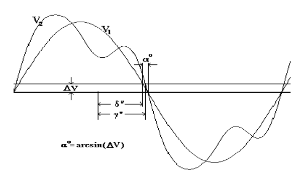
A medium voltage feeder serving a mix of residential and industrial customers has several capacitor banks along the feeder, not only for power factor correction but also for voltage control. It was hoped that by maintaining good voltages along the feeder there will be an increase of revenue. The capacitors were sized for summer loading when the load was high. The intention was to switch out some of the capacitor banks selectively during the fall when the load is much lighter. For some reason, all the capacitors remained connected when the fall season arrived. The line voltage went up to almost the allowed upper limit and caused all the distribution transformers on the feeder to go into the saturation region. The net effect was to cause all the uneven harmonics to increase. The additional voltage drop due to the high harmonic currents were sufficient to cause the feeder voltage to be heavily distorted. High precision motor drives that relied on accurate determination of the thyristor firing angles started to show erratic speeds. Many of the precision motor drives do not use the actual angle measured from the actual voltage zero crossing to determine the thyristor firing angle. Instead, it uses the voltage threshold level based on a pure 60 Hz sine wave to infer the firing angle magnitude. Referring to Figure 5 for illustration, the angular correction αo = arcsin (ΔV). For an angular setting of do the actual thyristor firing angle is (αo + δo). If the voltage is distorted then an error creeps in. The angular correction αo is now smaller. The harmonic distortion of the fundamental wave shifts the calculated angle with respect to the true voltage zero crossing and hence creates an error in angle measurements.
The obvious solution was to switch off some of the capacitor banks.
Figure 5
THE HIDDEN PROBLEMS
Accuracy of Energy Metering
Many papers have been written on the effects of harmonic distortion on energy metering. Even though the power quality standards tried to define the limits of distortion, there is still a need to standardize distortions for both currents and voltages, which can be used to calibrate energy meters. [4-6] There is a massive number of literature discussing this matter which is impossible to list in this paper. A few relevant ones are listed in the REFERENCE section.
This problem is becoming more acute with the influx of personal desk computers, quick start fluorescent lamps, energy saving lamps and thyristor controlled variable speed drives. They all generate non-linear load currents. In many cases the distorted load currents are large enough to cause voltage distortions at the metering points. Some of the smaller utilities are not aware about these customer generated power quality problems, especially if they do not cause problems to other customers. The loss of revenue due to errors in revenue metering is even less known. Even if the electric utility is aware about this problem, there is no place it can turn to for help in calibrating the meters for distorted waveforms.
Unbalance voltages
Unbalance in 3-phase systems not only causes problems with 3-phase rotating machines, but also with reactive power metering. A shortening of motor life due to operation under unbalance voltage conditions maybe more prevalent than what one dares to admit. Unfortunately no statistical data are available which correlates motor life to the degree of unbalance of the voltages. Combined with lower voltages, the problem becomes even worst. In areas with explosive growths, sometimes load growth was not followed by improvements of the distribution network. A changeover from a two-phase plus neutral to a three-phase system on the heavily loaded laterals are expensive. Each load site also requires an additional transformer and load balancing. It requires time to implement, not only by the electric utility but also by the energy user.
Effects of Harmonics
The effects of harmonics on motors/generators, transformers, power cables, capacitors, electronic equipment, metering, etc. are well documented. IEEE Std 519-1992 describes in general the harmful effects of these harmonics on the equipment. [1]. It also recommends practices for harmonic control and also set some limiting values for the harmonics not to exceed. Unfortunately no good standards of distortion for voltages, currents and phase angles commonly agreed to be used for calibration of different types of metering devices, for assessing incremental temperature rise in motors, etc. are available at this moment.
Some commercial customers and the electric utility serving these customers were not aware that harmonics were generated by the customers’ equipment themselves. These harmonics also cause damage to other equipment. An example was that of a high power television transmitter station. The transmitter tubes requires rectified dc voltages. The filter that came with the high voltage 6 phase rectifiers was never installed because it was deemed unnecessary by the installer of the television station. The distorted ac voltages were also used to operate the cooling pump motors and according to the station engineer, these pump motors have to be replaced after several months of operation. As a matter of fact he has several of these motors in stock for quick replacements of the damaged motors.
The accuracy of the energy metering was also questionable and the electric utility remained unaware about some revenue losses due to customer generated harmonics.
STANDARDS ISSUE
One of the most commonly encountered problems is the lack of standards on how much distortion a device can generate under operating conditions. A single equipment installed in a plant may cause insignificant amount of distortion. But when many of them are installed and in operation, the net total effects can be a problem for the plant and the individual device itself. The electric utility is only concerned about spillover effects that will harm other customers. If spillover is detected, it is difficult to get a measure of damage it may cause. It is even more difficult to express the damage in terms of dollars, especially when there is a need to institute a policy of penalizing the customer, which is the source of the harmonic pollution.
The incremental losses in the system due to harmonics, the loss in revenue, the reduced life of certain equipment, etc. though written about extensively in many professional magazines cannot be quantified and available methods remain elusive.
The currently available standards, excellent as they are in their own rights, are difficult to read and understand by most practicing engineers at the smaller utilities. What makes matters worse is the fact that the available power quality monitoring devices seemed to be designed for experts only.
There are no off the shelf energy meters that provide correction factors when operated under distorted voltage and current conditions. This is due to the fact that no standard for distortions exists that are accepted by the industry. Hence calibration standards cannot be started.
CONCLUSIONS
Our findings tell us that power quality problems are on the increase. We have indicated the variety of causes that lead to power quality problems. Some of them lend themselves to quick and low cost fixes. Others involve heavy capital investments by the electric utility as well as by the energy user. The electrical power industry may have to start something similar to Environmental Protection Agency in the USA. Policies have to be based on good and comprehensive standards defining limits of allowed unbalance and harmonic pollution. Also a method has to be devised for policing compliance and a measure for penalizing the guilty party needs to be developed. There may be also a need for some type of arbitration board to resolve the finger pointing issues.
Revenue metering is also affected by voltage and current distortions. Standards and calibration laboratories have to be developed for calibration of revenue meters.
There is also a need for life testing standards for equipment subjected to three phase unbalance voltages and voltage distortions.
Because of the highly competitive environment that deregulation has caused, the electric utilities are not only electric power providers but they also have to become service providers.
REFERENCES
[1] IEEE Standard 519-1992, “Recommended Practices and Requirements for Harmonic Control in Electrical Power Systems”, IEEE, New York, NY, 1993.
[2] IEEE Working Group on Nonsinusoidal Situations, “Practical Definitions for Powers in Systems with Nonsinusoidal Waveforms and Unbalanced Loads: A Discussion”, IEEE Trans. on Power Delivery, Vol. 11, No. 1, Jan. 1996, pp. 79-101.
[3] IEEE Standard 1159-1995, “IEEE Recommended Practice for Monitoring Electric Power Quality”, IEEE, New York, 1995.
[4] IEEE Working Group on Distribution Voltage Quality, “Guide on Service to Equipment Sensitive to Momentary Voltage Disturbances”, P1250/D4, Jan. 3, 1992.
[5] Y. Baghzouz, O. T. Tan, “Harmonic Analysis of Induction Watthour Meter Performance”, IEEE Trans. Power App. Syst., Vol. PAS-104, pp. 965- 969, Feb. 1985.
[6] R. Arseneau, P. S. Filipski, “Application of a Three Phase Nonsinusoidal Calibration System for Testing Energy and Demand Meters under Simulated Field Conditions”, IEEE Trans. on Power Delivery, Vol. PWRD-3 No. 2, July 1988, pp. 874-879.
[7] Westinghouse Electric Corporation, Electric Utility Engineering Reference Book-Distribution Systems, Vol. 3.
Published in 26th International Power System Conference, Oct 31st – Nov 2nd, 2011, Tehran, Iran.
Keywords-component; Harmonic Distortion, Loss estimation, Non-linear loads, Norton equivalent model, Power quality.
Abstract
This paper investigates the harmonic distortion and losses in distribution networks due to large number of nonlinear loads. These days the number of nonlinear loads in power systems is increasing dramatically. These nonlinear loads inject harmonic currents and voltages. Due to widespread usage of nonlinear loads in distribution systems, the harmonic distortion of the current and voltage increase. Power quality of distribution networks is severely affected due to the flow of harmonics. These harmonics can cause serious problems in power systems, excessive heat of appliances, components aging and capacity decrease, fault of protection and measurement devices, lower power factor and consequently reducing power system efficiency due to increasing losses are some main effects of harmonics in power distribution systems.
This paper investigates the amount of the harmonics caused by the nonlinear loads in residential, commercial and office loads and also estimates the loss of energy due to nonlinear loads harmonics. In order to analyze effects of nonlinear loads, electrical characteristics of more than 32 common nonlinear appliances are measured using a power quality analyzer set. In order to estimate harmonic distortions and losses in distribution networks a sample distribution network is modeled. The model follows a “bottom-up” approach, starting from calculating end users appliances Norton equivalent model and then modeling residential, commercial and office loads by synthesis process.
The presented harmonic Norton equivalent model of end users appliances is a simple and accurate model which is obtained based on the data from laboratory measurement results. Residential, commercial and office load types model is obtained by synthesis of their corresponding appliances and finally a sample distribution feeder in modeled by aggregating different types of loads. To study the harmonic distortions level and losses in distribution systems, a sample 20 kV/400 V feeder with nonlinear loads is simulated and increase in loss due to nonlinear loads is also estimated.
The simulations performed in MATLAB Simulink software. The proposed loss estimation method results are accurate and reliable because of the accurate modeling technique.
Introduction
In recent years, the use of nonlinear electronic loads such as compact fluorescent lamps (CFLs), computers, televisions, etc has increased significantly. Nonlinear loads inject harmonic currents into distribution network. When a combination of linear and nonlinear loads is fed from a sinusoidal supply, the total supply current will contain harmonics. Harmonics are currents or voltages with frequencies that are integer multiples of the fundamental power frequency. These harmonic currents and the corresponding resulted harmonic voltages can cause power quality problems and affect the performance of the consumers connected to the electric power network.
These harmonics can cause serious problems in power systems, excessive heat of appliances, components aging and capacity decrease, fault of protection and measurement devices, lower power factor and consequently reducing power system efficiency due to increasing losses are some main effects of harmonics in power distribution systems. Harmonic distortions can cause significant costs in distribution networks. Harmonic costs consist of harmonic energy losses, premature aging of electrical equipments and de-rating of equipments. The energy loss due to harmonics caused by billions of nonlinear loads used in different power system sectors could be predicted.
The difference between the known generation and the estimated consumption is considered as the energy loss. Although it is well known that there are many unauthorized consumers, there is no way to determine the technical (RI2 loss) and the commercial losses (various form of theft). Energy losses in distribution networks are generally estimated rather than measure, because of inadequate metering in these networks and also due to high cost of data collection. Moreover, power system distribution loss estimation methods are a reliable way to determine the technical losses. Accurate loss estimation plays an important role in determining the share of technical and commercial losses in the total loss. There are some works that estimated the losses in distribution systems by different methods. Some works use the simplified feeder models for computation of loss, and then use curve fitting approach to estimate the loss [1-5]. A comprehensive loss estimation method using detailed feeder and load models in a load-flow program is presented in [6]. A combination of statistical and load-flow methods is used to find various types of losses in a sample power system in [7]. Simulation of distribution feeders with load data estimated from typical customer load is performed in [8]. In [9] approximates are applied to power flow equations in order to estimate the losses under variations in power system components. A fuzzy based clustering method of losses and fuzzy regression technique and neural network technique for modeling the losses are obtained in [10, 11].
This work uses an accurate model for 20kv/400 v feeders to estimate distribution network losses. In this work different types of residential, commercial and office load are modeled using their appliances model by the process of synthesis and then a feeder model is obtained by aggregating different residential, commercial and office load type models. The appliances and consequently the residential, commercial and office loads are modeled by Norton equivalent technique. More than 32 nonlinear appliances are measured using a power quality analyzer set. The Norton model parameters for each appliance are calculated based on the measurements results of each load. The measurements are done on different operating conditions for deriving the Norton model parameters. More details about Norton equivalent model of appliances and loads is presented in [12-14].
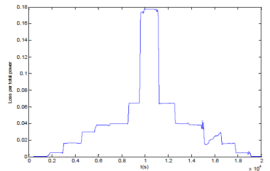
After analyzing the harmonic distortion levels in a modeled office load, a 20 kV/400 V feeder composed of residential, commercial and office loads are simulated and losses in transmission lines due to distorted current are discussed and also energy loss versus total transmitted power is calculated for the sample simulated feeder.
The paper is organized as follows. In Section II, harmonic power for nonlinear loads is introduced. In Section III, characteristics of some nonlinear appliances are presented and each type of the load harmonic distortion is investigated. In Section IV obtaining a Norton model for a nonlinear load based on measurement data is discussed. Section V introduces different loads type’s models and their simulation results. The losses due to nonlinear loads in a sample 20 kV/400 V feeder are simulated and analyzed in section VI. Finally, the conclusions are summarized in Section VII.
Harmonic Power for Nonlinear Loads
If a signal contains harmonics, the Individual Harmonic Distortion (IHD) for any harmonic order is defined as the percentage of the harmonic magnitude respect to the fundamental value.
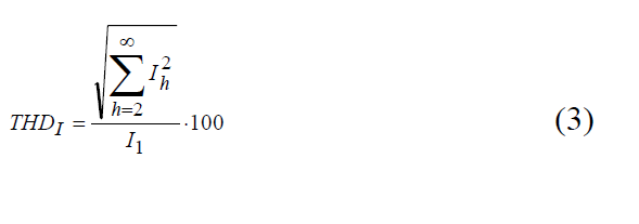
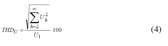
Nonetheless, for determining the level of harmonic content in an alternating signal, the term “Total Harmonic Distortion” (THD) of the current and voltage signals are used widely. THD according IEEE standards is defined as the ratio of the root-mean-square of the harmonic contents to the root-mean square value of the fundamental quantity, expressed as a percentage of the fundamental. So the current and voltage THD of a harmonic polluted waveform can be expressed as:
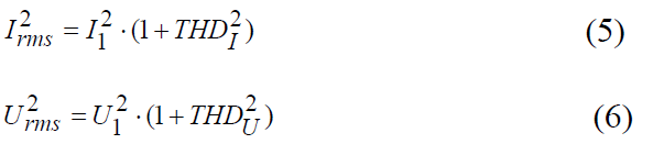
Since the numerators of the equations (3) and (4) are equal to the RMS values of the harmonic contents of voltage and current and respectively, these equations can be written as:
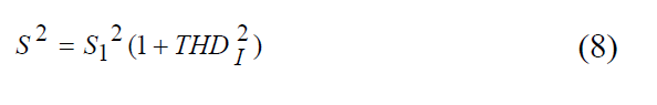
Equations (5) and (6) show that the RMS values of current and voltage for a harmonic polluted waveform are bigger than the fundamental value and this results in bigger apparent power.
The apparent power of a signal containing harmonics is calculated by the equation 7.
Since the THDU which comes through utility is much smaller than THDI in most cases, it can be ignored. Therefore,
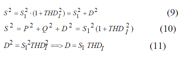
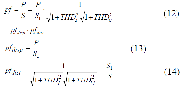
For a sinusoidal waveform, the apparent power S is comprised of active power P and reactive power Q, but presence of harmonics causes the presence of a new type of power, the Distortion Power D with units of voltamperes. Distortion power is described in following equations.
Power factor is not only affected by the phase displacement between voltage and current waveforms. The distortion power (D) also affects the power factor. Power factor will decrease in presence of harmonics and consequently distortion power (D).
In the case of presence of harmonics power factor is composed from two factors, Displacement Power Factor (pfdisp) and Distortion Power Factor (pfdist).
Nonlinear loads can be considered as harmonic real power sources that inject harmonic real power into the distribution system which is product of the harmonic voltage and harmonic current of the same orders. Although this power is much smaller than the fundamental real power, the presence of the distortion power caused by harmonics will result in increased losses flowing through the utility supply system.
For a linear load, the loss of the utility is I12R. With current distortion discussed above, the loss would be as:
So it can be seen that a significant increase in loss of the utility will be occurred in presence of harmonic distortions. For example, with a THDI=40%, the loss would be increased by 16%.
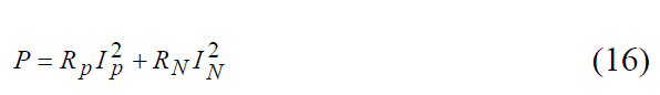
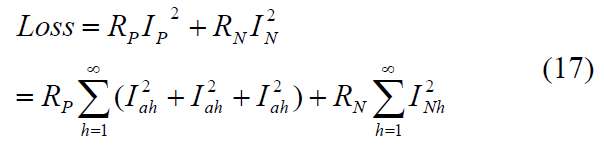
For a three-phase utility, the total losses are:
Where IP is the phase current of the balanced network and IN is the neutral line current. The harmonic losses are:
Where Iah, Ibh, and Ich are the order h harmonic currents in phase A, B and C respectively, and INh is the order h harmonic neutral current. RP and RN are the phase and neutral resistances. The loss of the neutral current can be considerable so that it can be the main part of the harmonic power loss. Two typical problems can overload the neutral conductor. One is unbalanced single phase loads and the other one occurs when the line to neutral voltage is badly distorted by the triple harmonic voltage drop in the neutral current [6].
Nonlinear loads and thier Charactristics
This section presents the measurement result for some very common residential and commercial appliances. The measurements consist of current and voltage THDS, rms value of current, power factor, active and reactive power. All the measurements are done by a HIOKI 9624 power quality analyzer.
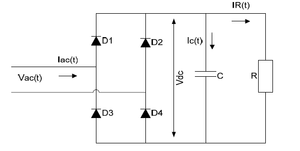
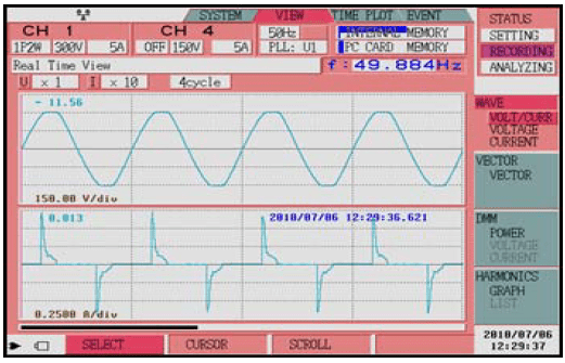
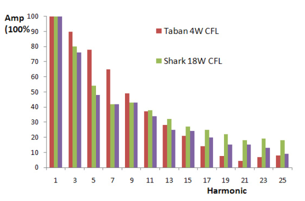
The simplified equivalent circuit of a CFL could be assumed as a rectifier with ideal switches and a capacitor in the DC link which supplies a resistor as shown in Fig. 1. The ac current waveform of a 4 W CFL as a nonlinear load is shown in the Fig. 2. In Fig. 3, the harmonic spectra are shown for some sample CFLs. The other nonlinear loads also inject non-sinusoidal currents when they are fed by a sinusoidal voltage. Some other nonlinear loads and their characteristics are listed in Table I.
Figure 1: Simplified CFL Circuit
Figure 2: Measured Current Waveform for a 4W CFL
Figure 3: Normalized Magnitude [%] Spectra Comparison for 3 different CFLs
Table I shows the electrical parameters for some linear and nonlinear appliances which are used in residential, commercial and office load types. Active and reactive power for each appliance is calculated and also distortion power (D) which has a nonzero value for nonlinear loads is calculated. Fortunately, the harmonic real power is much smaller that the fundamental real power. But, the harmonic current adds the distortion power (D) to apparent power (S). Therefore, the flow of the current will result in increased losses.
In this work power factor for all appliances is also measured and the effect of displacement and distortion factors on the total power factor is investigated. What follows is a summary of the measurements of the some appliances.
Table 1. Measurement results for some appliances
Load Type
THDI (%)
S1 (VA)
P1 ( W )
Q1 (Var)
D (Var)
PF
PFdisp
PFdist
CFL
155.00
8.06
4.00
-7.00
12.50
0.48
0.89
0.54
Fan
5.39
49.59
49.50
-2.96
2.67
0.99
0.99
1.00
Refrigerator
15.53
130.59
106.95
74.93
20.28
0.80
0.81
0.99
Computer
114.05
152.20
95.91
-118.18
173.59
0.63
0.95
0.66
Laptop
159.60
51.82
26.00
-44.83
82.71
0.50
0.94
0.53
Television
142.73
93.47
49.60
-79.23
133.42
0.53
0.92
0.57
Washing machine
2.42
2072.28
2072.2
-12.31
50.15
0.48
0.48
1.00
Vacuum
21.97
1024.94
987.36
275.00
225.18
0.96
0.99
0.98
Iron
2.96
1119.60
1119.4
-21.00
33.17
1.00
1.00
1.00
Blow dryer(Slow Rate)
8.43
526.76
525.00
43.00
44.42
1.00
1.00
1.00
Blow dryer(Fast Rate)
3.15
980.17
980.00
18.00
30.88
1.00
1.00
1.00
freezer
9.69
313.37
217.79
225.32
30.36
0.69
0.70
1.00
Fluorescent lamp
8.23
74.78
28.95
68.95
6.16
0.38
0.39
1.00
Incandescent lamp
2.83
96.17
96.10
-3.70
2.72
1.00
1.00
1.00
Split air conditioner
22.54
2692.15
1834.4
1970.4
606.81
0.87
0.89
0.98
air conditioner
23.96
1417.91
1032.3
972.00
339.73
0.94
0.97
0.97
Norton Equivalent Model
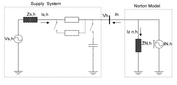
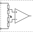
To obtain a Norton model for a nonlinear load, the circuit shown in Fig. 5 can be used [7, 8]. In this circuit the supply side is represented by the Thevenin equivalent while the nonlinear load side is represented by the Norton equivalent. For calculating the Norton model parameters, measurement of voltage (Vh) and current (Ih) spectra for two different operating conditions of the supply system are needed. The change in the supply system operating condition can for example be obtained by switching a shunt capacitor, a parallel transformer, shunt impedance or some other changes that cause a change in the supply system harmonic impedance [7, 8]. However, such changes in supply system will not yield unique parameters for the Norton model, and the Model parameters are dependent on the amount of change. This makes the accuracy of the model debatable. In [9], it is shown that the Norton model parameters which are obtained by changing the supply voltage are more accurate and valid for a wider range of voltage variations. Also, changing the supply voltage, beside its simplicity, does not require switching large capacitors or impedances which may cause some problems for network components.
As Fig. 4 shows, when the supply voltage varies, harmonic voltage Vh and harmonic current Ih will change and IN,h finds a path which consists of a parallel combination of ZN,h and the supply system impedance. With the assumption of no change in the operating conditions of the nonlinear load, it can be seen from Fig. 4 that Ih,1 and Ih,2 can be expressed as:
Figure 4: Norton Model of Load-Side and Thevenin Equivalent of Supply System [7]
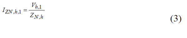
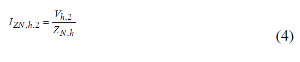
The harmonic Norton impedance current IZN,h , before and after the change can be expressed as:
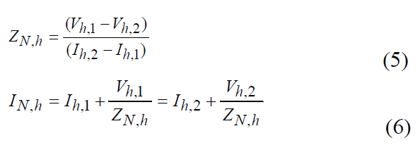
By substituting Eqs. 3 and 4 in Eqs. 1 and 2 and solving for ZN,h and IN,h the following formulas are achieved [8]:
where Vh,1 and Ih,1 are the harmonic voltage and current measurements before the change in the operating condition, and Vh,2 and Ih,2 are the measurements after the change. Note that these equations are complex and moreover the voltage and current magnitudes, their phase angles also should be measured precisely. In the following section, a Norton model is developed for CFLs based on Norton parameters, and the proposed model is compared with the measurement results.
Residential, Commercial and Office loads Norton Equivalent Model
In this section a model for residential, commercial and office loads is developed based on aggregating their corresponding appliances models. To develop the Norton model for each appliance at least two measurements at different operating condition of the supply system are needed. More details about how to achieve the Norton equivalent model parameters using measurement results is described in previous section and [12-14] and 17.
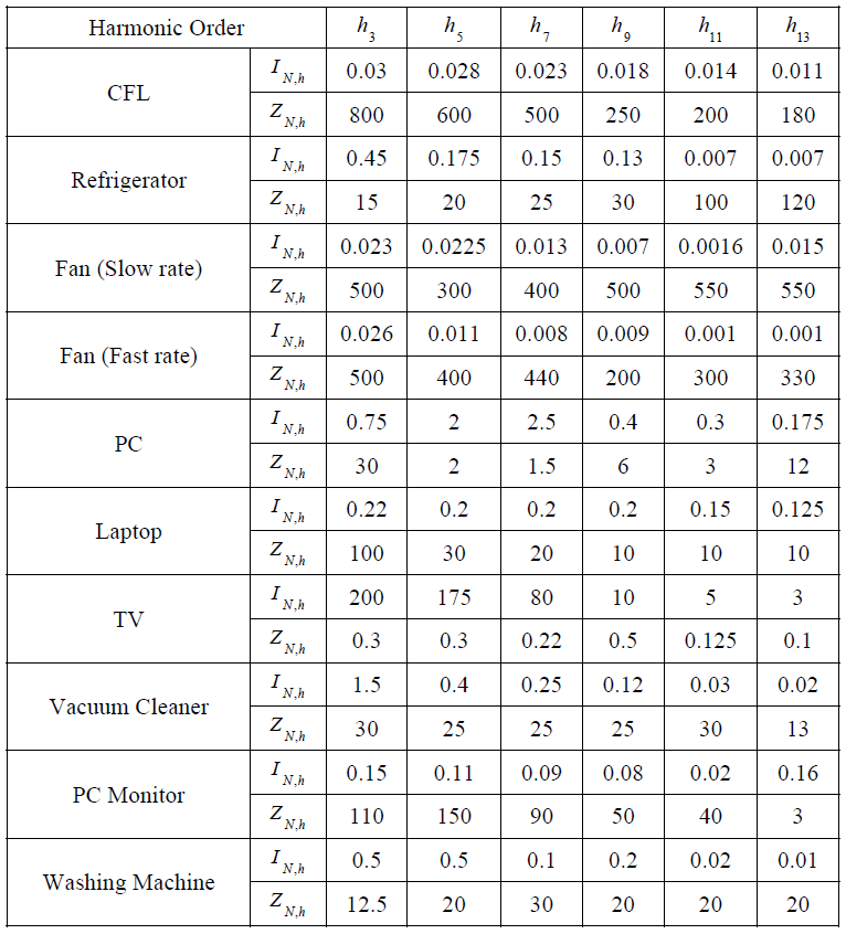
Norton equivalent model parameters consist of ZN and IN for each harmonic order. The Norton equivalent model is developed for each harmonic order separately, and the complete Norton equivalent model is obtained by combining these models. The Norton model parameters for different residential loads are given in the Table. II.
Table 2. Norton Model Parameters for Residential appliances
In this work, more than two different operating conditions are considered to obtain better modeling results. The measurement has done at more than two hundred different operating conditions of the supply voltage. The achieved Norton equivalent current and impedances values in different operating conditions converged to a specific value. This convergent make the achieved results more reliable.
After modeling each appliance, residential, commercial and office loads Norton equivalent model will be achieved by aggregating their corresponding appliances Norton equivalent models. In next level a feeder Norton equivalent model will be obtained by aggregating a residential, commercial and office load Norton equivalent models.
Simulation results for a 20 kV Distribution Network
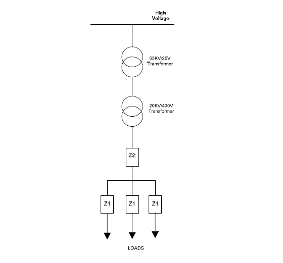
This section analyses the characteristics of a sample distribution network feeder modeled by Norton equivalent technique. This feeder model is obtained based on aggregating the Norton equivalent model of all end user appliances. Obtaining Norton equivalent model of appliances is more described in [14]. A simple schematic for a simple 3 phase balanced distribution network is shown in figure 5 .As figure 5 shows the sample feeder feeds 3 different loads (residential, commercial, office). The total feeder load is equal to the sum of all 3 loads. In this section, a sample office load model and its characteristics are investigated specifically and then characteristics of a feeder composed of residential, commercial, office load models is investigated.
Figure 5: Schematic of a sample 20kV/400V feeder
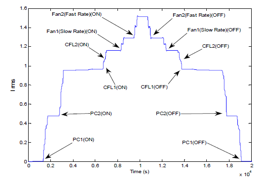
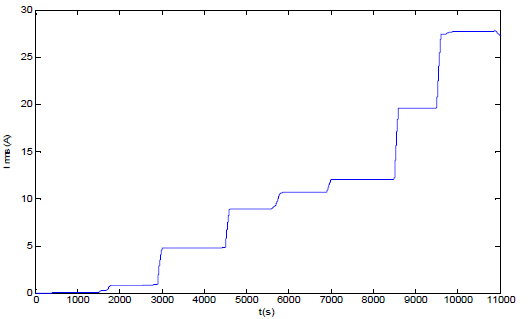
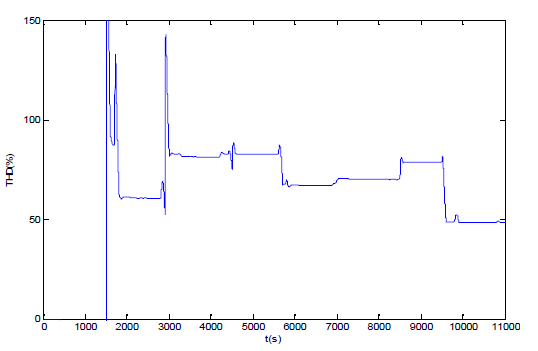
Using the models for each appliance, an estimation of the power quality of a customer can now be obtained. The assumed office load is supposed to have 2 PCs, 2 CFLs and 2 fans with slow and fast rates. The loads turn on one by one. Figs. 6 and 7 show the rms current and THD of the office load. The point of turning on or off for each appliance is shown in Fig.6.
Figure 6: Simulated office load rms current
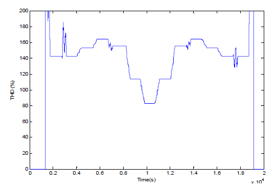
Figure 7: THD trend for simulated office load
The Total Harmonic Distortion (THD) of the office load depends on each appliance THD and its rms value of current. As Figs. 6 and 7 shows the THD decrease as the load current increase.
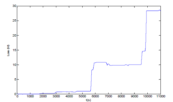
It is assumed that a 20 KV feeder feeds three different types of residential, commercial and office loads. Each load appliances are as Table.3 shows.
Table 3. Simulated residential, commercial and office loads appliances
Load type
Appliances
Residential
2 CFLs, Refrigerator, TV, Washing Machine, Vacuum, Iron, Fan
Office
2 PCs, 2CFLs, Laptop, TV, Refrigerator, Printer, Fan
Commercial
2 CFLs, TV, Fan, PC
The appliances turn on one by one and finally all of the appliances are in on state. Fig. 8 shows the feeder total rms current trend from the starting time up to the time that all of the appliances are turned on.
Figure 8: Simulated feeder total current
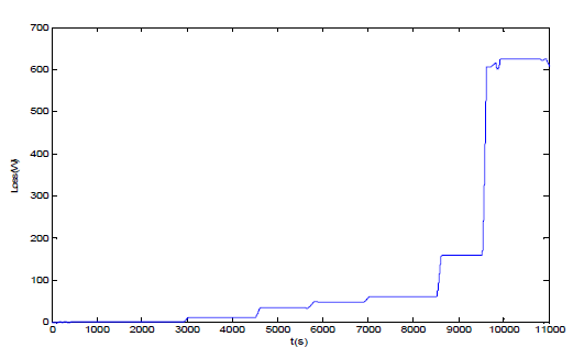
Figure 9: Simulated feeder Total Harmonic Distortion
Figure 9 shows the total harmonic distortion of the feeder current. As this figure shows the THD varies when different appliances turn on. The effect of each appliance on the total feeder THD is dependent on the each appliance THD and its current rms value.
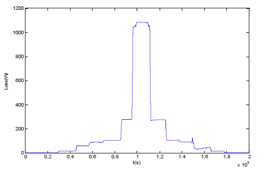
Losses in 20 kV Distribution Networks
In this section losses in transmission lines for the simulated distribution network in section VI are calculated using the equations introduced in section II. Schematic of a sample feeder in figure 5 contains two impedances for the transmission lines (Z1 and Z2). Figure 10 shows the losses due to Z1 impedance for an office load and figure 11 shows losses due to Z2 impedance that three feeder loads current flow through this impedance. As this figures show the loss values increase when the loads turn on and accordingly the lines current increases. The peak value of loss in achieved when all the appliances are turned on. Z1 and Z2 resistances are considered 1 ohm and inductive impedances are neglected.
Figure 10: Losses in Z1 impedance for and office load
Figure 11: losses in Z2 impedance which feeds three loads
Total loss in Z1 and Z2 impedances for the simulated feeder is shown in figure 12. As Fig.12 shows the loss behavior is similar to the aggregated loads rms current.
Figure 12: Total losses in Z1 and Z2 impedances
Total amount of losses in this sample feeder reaches to 1100 watt in the maximum stage. This amount of losses versus the total feeder load is plotted in figure 13.
Figure 13: Real power loss versus total feeder real power
The loss in distribution systems is related with the square of the current and this can be seen in the above figures. When the feeder current reaches to its maximum value, the losses value increase in a faster rate and this is because of the quadratic relationship between loss and current.
Losses due to transmission lines impedance for the simulated power network could be increased to 18% of the total feeder power and this amount of loss means a considerable cost for distribution networks that could not be neglected.
Share of nonlinear loads and their harmonics in causing loss of power in distribution networks could be obtained by the equation 15. According to the figure 9, if the average Total Harmonic Distortion (THD) of the sample power distribution network be considered 50%, then share of the harmonics losses in total losses will be equal to 20% of total loss.
Conclusions
In this paper, a comprehensive investigation has been investigated to determine the effects of harmonic distortions on power system distribution networks. Harmonics due to widespread usage of nonlinear increased recently so that returning to linear load conditions will remain a dream in feature. This work used the Norton equivalent model of different appliances which are obtained by the analyzing the measurement results. Distortion power is defined for common appliances and effect of harmonics on appliances power factor is detailed. The results are reasonably accurate because the Norton equivalent models are pierce and obtained based on the measurements results. Different load type models are achieved by aggregating the Norton equivalent model of individual appliances. A sample feeder is modeled using different residential, commercial and office loads model and losses due to transmission losses are investigated and also share of harmonics in causing extra losses are determined. The results shows that the losses can be increased to 18% percent of the feeder real power and the share of harmonics in these losses is dependent to the total harmonic distortion of the feeder current waveform.
Acknowledgment
The authors of this paper would like to thank Iran Energy Efficiency Organization (IEEOSABA) for their supports in carrying out this research.
References
[1] F. H. Buller and C. A. Woodrow, “Load factor equivalent hours values compared,” Electr. World, Jul. 1928.
[2] H. F. Hoebel, “Cost of electric distribution losses,” Electr. Light and Power, Mar. 1959.
[3] M.W. Gustafson, J. S. Baylor, and S. S. Mulnix, “Equivalent hours loss factor revisited,” IEEE Trans. Power Syst., vol. 3, no. 4, pp. 1502–1507, Nov. 1988.
[4] M.W. Gustafson, “Demand, energy and marginal electric system losses,” IEEE Trans. Power App. Syst., vol. PAS-102, no. 9, pp. 3189–3195, Sep. 1983.
[5] M.W. Gustafson and J. S. Baylor, “Approximating the system losses equation,” IEEE Trans. Power Syst., vol. 4, no. 3, pp. 850–855, Aug. 1989.
[6] D. I. H. Sun, S. Abe, R. R. Shoults, M. S. Chen, P. Eichenberger, and D. Ferris, “Calculation of energy losses in a distribution system,” IEEE Trans. Power App. Syst., vol. PAS-99, no. 4, pp. 1347– 1356, Jul./Aug. 1980.
[7] R. Céspedes, H. Durán, H. Hernández, and A. Rodríguez, “Assessment of electrical energy losses in the Colombian power system,” IEEE Trans. Power App. Syst., vol. PAS-102, no. 11, pp. 3509– 3515, Nov. 1983.
[8] C. S. Chen, M. Y. Cho, and Y.W. Chen, “Development of simplified loss models for distribution system analysis,” IEEE Trans. Power Del., vol. 9, no. 3, pp. 1545–1551, Jul. 1994.
[9] O.M. Mikic, “Variance Based Energy Loss Comptation in LV Distribution Networks”. IEEE Trans. Power Syst., vol. 22, no. 1, pp. 179-187, Feb. 2007.
[10] C.S.Chen, C.H.Lin, “Development of Distribution Feeder Loss Models by Artificial Neural Networks”, IEEE Conference, 2005, Taiwan.
[11]Y.-Y. Hong and Z.-T. Chao, “Development of energy loss formula for distribution systems using FCN algorithm and cluster-wise fuzzy regression,” IEEE Trans. Power Del., vol. 17, no. 3, pp. 794–799, Jul. 2002.
[12]Thunberg, E. and Söder, L., “A Norton Approach to Distribution Network Modeling for Harmonic Studies”, IEEE Trans. Power Delivery, Vol.14, No.1, pp. 272-277, January, 1999.
[13]Thunberg, E. and Söder, L., “On the Performance of a Distribution Network Harmonic Norton Model”, ICHQP 2000, Florida, USA, 01-04 October, 2000.
[14]Abdelkader, S., Abdel-Rahman, M.H., Osman, M.G., “A Norton equivalent model for nonlinear loads”, LESCOPE conference, Halifax, Canada, july, 2001.
[15]Balci, M.E., Ozturk, D., Karacasu, O., Hocaoglu, M.H., “Experimental Verification of Harmonic Load Models”, UPEC conference, Padova, September, 2008.
[16]Jing Yong, Liang Chen, Nassif, A.B., Wilsun Xu, “A Frequency-Domain Model for Compact Fluorescent Lamps”, IEEE Trans. Power Delivery, Vol.25, No.2, pp. 1182-1189, April, 2010. M.J.Ghorbani, H.Mokhtari,”Residential load modeling by Norton Equivalent Model of household loads”, APPEEC 2011, China, 2011.
1. A new revision of the IEC standard for PQ monitors 61000-4-30 Class Edition 3 2015 has been released.
Why?
It includes new parameters and new requirements for accuracy over the entire operating temperature range.
2. The PQ Instrument must have 4 each differential voltage and 4 differential current channels.
(Differential means two connections per channel high and low. ) Some power monitor instruments are equipped with a single ended (non-differential input). A differential input channel is not referenced to ground, but both sides of the input are “floating”.
Differential
NOT Single-ended
Where the voltage or current that is measured with this single ended inputs is always measured between that specific point and ground.
Why?
Without differential voltage channels, ALL voltage measurements are made relative to ground. This means measurements in an AC Delta circuit require a ground connection. But a power transformer delta output is not referenced to ground! So the measurement results will have unknown errors because of ground potential rise. For example during a fault or during a lightning strike. The result is invalid data.
3. All parameters, on all channels must be recorded synchronized and simultaneously in all modes all the time. This means the instrument records all the parameters and the user chooses which parameters to view after the recording period.
Why?
If the user has to select the parameters to be recorded before starting the recording, he is forced to guess what parameters are required for this site. If he guesses wrong, then the recording time is wasted and he’ll have to do it again.
4. All parameters must be sampled at the same frequency regardless of the monitor mode, setup or duration of monitoring period.
Why?
This is required to provide consistent data for analysis and comparison between voltage levels or different points on the network. It’s also required in the event a dispute between the utility and the user. Because different sample frequencies mean different resolution on time of event and possible gaps in the data when the instrument is “blind”. (not sampling). How can user decide which is needed for each site to be surveyed.
5. The instrument must have an enunciator type displaying the QOS (Quality of supply) while monitoring. This display must show the current state of the Quality of Supply real time of voltage, current, frequency, imbalance, swells, sag events, transients, flicker, THD without disrupting monitoring.
Why?
So the user ( or even none experienced user) can determine very quickly at any time during the monitoring the status of the Quality of Supply without transfering data to a computer or even touching the instrument.
6. The instrument must be capable of automatically testing the wiring connections for errors and alerting the user to the situation automatically.
Why?
To correct any connection errors before monitoring
7. The instrument must be have built-in software to analyze voltage events and catagorize them per the IEC or IEEE International standards.
Why?
So the report generated identifies the PQ incidents compared to the IEEE or IEC standard automatically.
8. Software must include the capability for the user to correct connection errors, time of day errors and align the time stamps of data taken by separate monitors.
Why?
So user can correct the data and prepare the report without having to repeat the monitoring, using the existing data file.
9. Software must include the capability to post process the periodic waveform event data and determine the individual voltage, current , power harmonics and interharmonics to the 125th harmonic.
Why?
This is advanced capability to provide additional data analysis from waveforms recorded during the monitoring period
10. Software must provide the capability to calculate TDD (Total Demand Distortion) and Even/ODD THD.
Why?
In the case where the instrument does not have these calculations built in.
11. Software must include the capability automatically generate reports to International standards and allow the user to define their own standard.
Why?
Reduce the engineering time to generate reports that are complete and easily understood.
12. Software must include the capability to calculate additional parameters for the recorded data , such as a virtual neutral current.
Why?
It gives the user the option of using the 4th current channel to monitor ground current
PQView 4brings you a smooth interface for viewing PQDIF and COMTRADE files, along with a wealthof other power quality monitoring and analytical capabilities. But what if you’re in a pinch and only need the file viewer?
PQDiffractor is a PQDIF and COMTRADE viewer written byElectrotek Concepts, Inc.for viewing, browsing, diagnosing, and converting PQDIF files and COMTRADE files, and is a free software download from our website.
That’s right. It’s free.
Read binary PQDIF Files using specifications from IEEE Std 1159.3-2003
Read ASCII or binary COMTRADE Files using specifications from IEEE Std C37.111-1991 or C37.111-1999
View lists of data source records in each PQDIF file
View lists of analog and digital channels from COMTRADE configuration files
Create interactive charts from PQDIF observations with channels of any quantity type
View samples from analog COMTRADE waveforms and digital status channels
Export displayed observations to Microsoft Excel as CSV files
To read more about PQDIF and COMTRADE, and to view a full list of PQDiffractor’s capabilities, visit our website, at electrotek.com/pqdiffractor/