Published by
Mohammad Jawad Ghorbani, Salar Atashpar, Arash Mehrafrooz, Iran Energy Efficiency Organization (IEEO), Tehran, Iran.
Emails: mjghorbany@ee.sharif.edu, s_atashpar@yahoo.com, arashmehrafrooz@saba.org.ir,
Hossein Mokhtari, Sharif University of Tech, Tehran, Iran.
Email: Mokhtari@sharif.edu
Published in 26th International Power System Conference, Oct 31st – Nov 2nd, 2011, Tehran, Iran.
Keywords-component; Harmonic Distortion, Loss estimation, Non-linear loads, Norton equivalent model, Power quality.
Abstract
This paper investigates the harmonic distortion and losses in distribution networks due to large number of nonlinear loads. These days the number of nonlinear loads in power systems is increasing dramatically. These nonlinear loads inject harmonic currents and voltages. Due to widespread usage of nonlinear loads in distribution systems, the harmonic distortion of the current and voltage increase. Power quality of distribution networks is severely affected due to the flow of harmonics. These harmonics can cause serious problems in power systems, excessive heat of appliances, components aging and capacity decrease, fault of protection and measurement devices, lower power factor and consequently reducing power system efficiency due to increasing losses are some main effects of harmonics in power distribution systems.
This paper investigates the amount of the harmonics caused by the nonlinear loads in residential, commercial and office loads and also estimates the loss of energy due to nonlinear loads harmonics. In order to analyze effects of nonlinear loads, electrical characteristics of more than 32 common nonlinear appliances are measured using a power quality analyzer set. In order to estimate harmonic distortions and losses in distribution networks a sample distribution network is modeled. The model follows a “bottom-up” approach, starting from calculating end users appliances Norton equivalent model and then modeling residential, commercial and office loads by
synthesis process.
The presented harmonic Norton equivalent model of end users appliances is a simple and accurate model which is obtained based on the data from
laboratory measurement results. Residential, commercial and office load types model is obtained by synthesis of their corresponding appliances and finally a sample distribution feeder in modeled by aggregating different types of loads. To study the harmonic distortions level and losses in distribution systems, a sample 20 kV/400 V feeder with nonlinear loads is simulated and increase in loss due to nonlinear loads is also estimated.
The simulations performed in MATLAB Simulink software. The proposed loss estimation method results are accurate and reliable because of the accurate modeling technique.
Introduction
In recent years, the use of nonlinear electronic loads such as compact fluorescent lamps (CFLs), computers, televisions, etc has increased significantly. Nonlinear loads inject harmonic currents into distribution network. When a combination of linear and nonlinear loads is fed from a sinusoidal supply, the total supply current will contain harmonics. Harmonics are currents or voltages with frequencies that are integer multiples of the fundamental power frequency. These harmonic currents and the corresponding resulted harmonic voltages can cause power quality problems and affect the performance of the consumers connected to the electric power network.
These harmonics can cause serious problems in power systems, excessive heat of appliances, components aging and capacity decrease, fault of protection and measurement devices, lower power factor and consequently reducing power system efficiency due to increasing losses are some main effects of harmonics in power distribution systems. Harmonic distortions can cause significant costs in distribution networks. Harmonic costs consist of harmonic energy losses, premature aging of electrical equipments and de-rating of equipments. The energy loss due to harmonics caused by billions of nonlinear loads used in different power system sectors could be predicted.
The difference between the known generation and the estimated consumption is considered as the energy loss. Although it is well known that there are many unauthorized consumers, there is no way to determine the technical (RI2 loss) and the commercial losses (various form of theft). Energy losses in distribution networks are generally estimated rather than measure, because of inadequate metering in these networks and also due to high cost of data collection. Moreover, power system distribution loss estimation methods are a reliable way to determine the technical losses. Accurate loss estimation plays an important role in determining the share of technical and commercial losses in the total loss. There are some works that estimated the losses in distribution systems by different methods. Some works use the simplified feeder models for computation of loss, and then use curve fitting approach to estimate the loss [1-5]. A comprehensive loss estimation method using detailed feeder and load models in a load-flow program is presented in [6]. A combination of statistical and load-flow methods is used to find various types of losses in a sample power system in [7]. Simulation of distribution feeders with load data estimated from typical customer load is performed in [8]. In [9] approximates are applied to power flow equations in order to estimate the losses under variations in power system components. A fuzzy based clustering method of losses and fuzzy regression technique and neural network technique for modeling the losses are obtained in [10, 11].
This work uses an accurate model for 20kv/400 v feeders to estimate distribution network losses. In this work different types of residential, commercial and office load are modeled using their appliances model by the process of synthesis and then a feeder model is obtained by aggregating different residential, commercial and office load type models. The appliances and consequently the residential, commercial and office loads are modeled by Norton equivalent technique. More than 32 nonlinear appliances are measured using a power quality analyzer set. The Norton model parameters for each appliance are calculated based on the measurements results of each load. The measurements are done on different operating conditions for deriving the Norton model parameters. More details about Norton equivalent model of appliances and loads is presented in [12-14].
After analyzing the harmonic distortion levels in a modeled office load, a 20 kV/400 V feeder composed of residential, commercial and office loads are simulated and losses in transmission lines due to distorted current are discussed and also energy loss versus total transmitted power is calculated for the sample simulated feeder.
The paper is organized as follows. In Section II, harmonic power for nonlinear loads is introduced. In Section III, characteristics of some nonlinear appliances are presented and each type of the load harmonic distortion is investigated. In Section IV obtaining a Norton model for a nonlinear load based on measurement data is discussed. Section V introduces different loads type’s models and their simulation results. The losses due to nonlinear loads in a sample 20 kV/400 V feeder are simulated and analyzed in section VI. Finally, the conclusions are summarized in Section VII.
Harmonic Power for Nonlinear Loads
If a signal contains harmonics, the Individual Harmonic Distortion (IHD) for any harmonic order is defined as the percentage of the harmonic magnitude respect to the fundamental value.

Nonetheless, for determining the level of harmonic content in an alternating signal, the term “Total Harmonic Distortion” (THD) of the current and voltage signals are used widely. THD according IEEE standards is defined as the ratio of the root-mean-square of the harmonic contents to the root-mean square value of the fundamental quantity, expressed as a percentage of the fundamental. So the current and voltage THD of a harmonic polluted waveform can be expressed as:
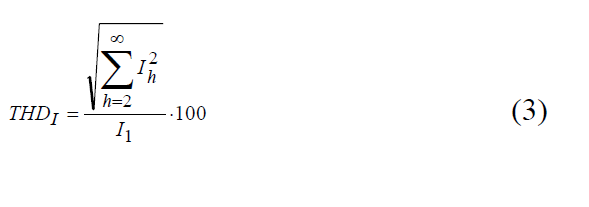
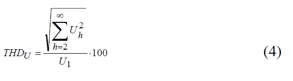
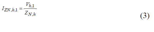
Since the numerators of the equations (3) and (4) are equal to the RMS values of the harmonic contents of voltage and current and respectively, these equations can be written as:
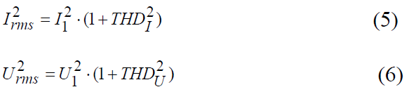
Equations (5) and (6) show that the RMS values of current and voltage for a harmonic polluted waveform are bigger than the fundamental value and this results in bigger apparent power.
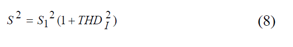
The apparent power of a signal containing harmonics is calculated by the equation 7.

Since the THDU which comes through utility is much smaller than THDI in most cases, it can be ignored. Therefore,
For a sinusoidal waveform, the apparent power S is comprised of active power P and reactive power Q, but presence of harmonics causes the presence of a new type of power, the Distortion Power D with units of voltamperes. Distortion power is described in following equations.
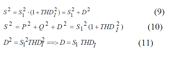
Power factor is not only affected by the phase displacement between voltage and current waveforms. The distortion power (D) also affects the power factor. Power factor will decrease in presence of harmonics and consequently distortion power (D).
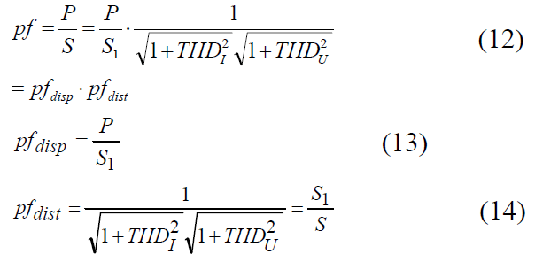
In the case of presence of harmonics power factor is composed from two factors, Displacement Power Factor (pfdisp) and Distortion Power Factor (pfdist).
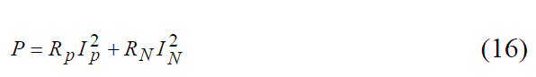
Nonlinear loads can be considered as harmonic real power sources that inject harmonic real power into the distribution system which is product of the harmonic voltage and harmonic current of the same orders. Although this power is much smaller than the fundamental real power, the presence of the distortion power caused by harmonics will result in increased losses flowing through the utility supply system.
For a linear load, the loss of the utility is I12R. With current distortion discussed above, the
loss would be as:

So it can be seen that a significant increase in loss of the utility will be occurred in presence of harmonic distortions. For example, with a THDI=40%, the loss would be increased by 16%.
For a three-phase utility, the total losses are:
Where IP is the phase current of the balanced network and IN is the neutral line current. The harmonic losses are:
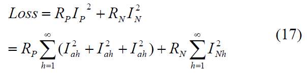
Where Iah, Ibh, and Ich are the order h harmonic currents in phase A, B and C respectively, and INh is the order h harmonic neutral current. RP and RN are the phase and neutral resistances. The loss of the neutral current can be considerable so that it can be the main part of the harmonic power loss. Two typical problems can overload the neutral conductor. One is unbalanced single phase loads and the other one occurs when the line to neutral voltage is badly distorted by the triple harmonic voltage drop in the neutral current [6].
Nonlinear loads and thier Charactristics
This section presents the measurement result for some very common residential and commercial appliances. The measurements consist of current and voltage THDS, rms
value of current, power factor, active and reactive power. All the measurements are done by a HIOKI 9624 power quality analyzer.
The simplified equivalent circuit of a CFL could be assumed as a rectifier with ideal switches and a capacitor in the DC link which supplies a resistor as shown in Fig. 1. The ac current waveform of a 4 W CFL as a nonlinear load is shown in the Fig. 2. In Fig. 3, the harmonic spectra are shown for some sample CFLs. The other nonlinear loads also inject non-sinusoidal currents when they are fed by a sinusoidal voltage. Some other nonlinear loads and their characteristics are listed in Table I.
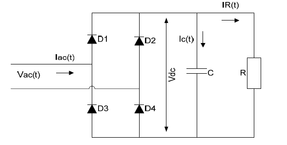
Figure 1: Simplified CFL Circuit
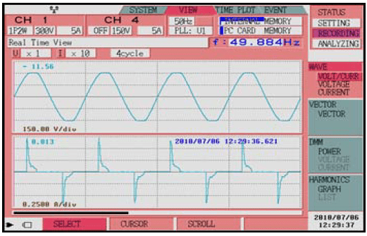
Figure 2: Measured Current Waveform for a 4W CFL
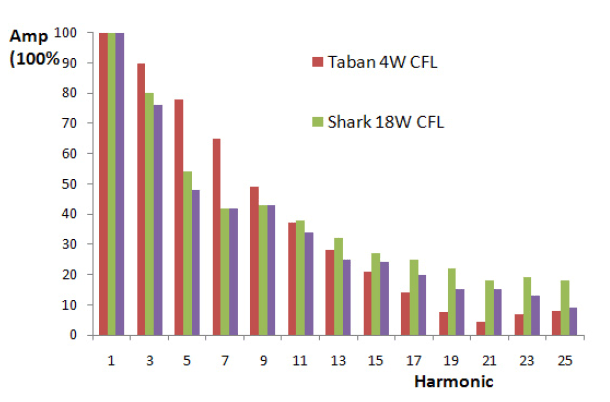
Figure 3: Normalized Magnitude [%] Spectra Comparison for 3 different CFLs
Table I shows the electrical parameters for some linear and nonlinear appliances which are used in residential, commercial and office load types. Active and reactive power for each appliance is calculated and also distortion power (D) which has a nonzero value for nonlinear loads is calculated. Fortunately, the harmonic real power is much smaller that the fundamental real power. But, the harmonic current adds the distortion power (D) to apparent power (S). Therefore, the flow of the current will result in increased losses.
In this work power factor for all appliances is also measured and the effect of displacement and distortion factors on the total power factor is investigated. What follows is a summary of the measurements of the some appliances.
Table 1. Measurement results for some appliances
| Load Type | THDI (%) | S1 (VA) | P1 ( W ) | Q1 (Var) | D (Var) | PF | PFdisp | PFdist |
|---|---|---|---|---|---|---|---|---|
| CFL | 155.00 | 8.06 | 4.00 | -7.00 | 12.50 | 0.48 | 0.89 | 0.54 |
| Fan | 5.39 | 49.59 | 49.50 | -2.96 | 2.67 | 0.99 | 0.99 | 1.00 |
| Refrigerator | 15.53 | 130.59 | 106.95 | 74.93 | 20.28 | 0.80 | 0.81 | 0.99 |
| Computer | 114.05 | 152.20 | 95.91 | -118.18 | 173.59 | 0.63 | 0.95 | 0.66 |
| Laptop | 159.60 | 51.82 | 26.00 | -44.83 | 82.71 | 0.50 | 0.94 | 0.53 |
| Television | 142.73 | 93.47 | 49.60 | -79.23 | 133.42 | 0.53 | 0.92 | 0.57 |
| Washing machine | 2.42 | 2072.28 | 2072.2 | -12.31 | 50.15 | 0.48 | 0.48 | 1.00 |
| Vacuum | 21.97 | 1024.94 | 987.36 | 275.00 | 225.18 | 0.96 | 0.99 | 0.98 |
| Iron | 2.96 | 1119.60 | 1119.4 | -21.00 | 33.17 | 1.00 | 1.00 | 1.00 |
| Blow dryer(Slow Rate) | 8.43 | 526.76 | 525.00 | 43.00 | 44.42 | 1.00 | 1.00 | 1.00 |
| Blow dryer(Fast Rate) | 3.15 | 980.17 | 980.00 | 18.00 | 30.88 | 1.00 | 1.00 | 1.00 |
| freezer | 9.69 | 313.37 | 217.79 | 225.32 | 30.36 | 0.69 | 0.70 | 1.00 |
| Fluorescent lamp | 8.23 | 74.78 | 28.95 | 68.95 | 6.16 | 0.38 | 0.39 | 1.00 |
| Incandescent lamp | 2.83 | 96.17 | 96.10 | -3.70 | 2.72 | 1.00 | 1.00 | 1.00 |
| Split air conditioner | 22.54 | 2692.15 | 1834.4 | 1970.4 | 606.81 | 0.87 | 0.89 | 0.98 |
| air conditioner | 23.96 | 1417.91 | 1032.3 | 972.00 | 339.73 | 0.94 | 0.97 | 0.97 |
Norton Equivalent Model
To obtain a Norton model for a nonlinear load, the circuit shown in Fig. 5 can be used [7, 8]. In this circuit the supply side is represented by the Thevenin equivalent while the nonlinear load side is represented by the Norton equivalent. For calculating the Norton model parameters, measurement of voltage (Vh) and current (Ih) spectra for two different operating conditions of the supply system are needed. The change in the supply system operating condition can for example be obtained by switching a shunt capacitor, a parallel transformer, shunt impedance or some other changes that cause a change in the supply system harmonic impedance [7, 8]. However, such changes in supply system will not yield unique parameters for the Norton model, and the Model parameters are dependent on the amount of change. This makes the accuracy of the model debatable. In [9], it is shown that the Norton model parameters which are obtained by changing the supply voltage are more accurate and valid for a wider range of voltage variations. Also, changing the supply voltage, beside its simplicity, does not require switching large capacitors or impedances which may cause some problems for network components.
As Fig. 4 shows, when the supply voltage varies, harmonic voltage Vh and harmonic current Ih will change and IN,h finds a path which consists of a parallel combination of ZN,h and the supply system impedance. With the assumption of no change in the operating conditions of the nonlinear load, it can be seen from Fig. 4 that Ih,1 and Ih,2 can be expressed as:

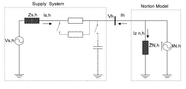
Figure 4: Norton Model of Load-Side and Thevenin Equivalent of Supply System [7]
The harmonic Norton impedance current IZN,h , before and after the change can be expressed as:
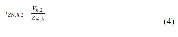
By substituting Eqs. 3 and 4 in Eqs. 1 and 2 and solving for ZN,h and IN,h the following formulas are achieved [8]:
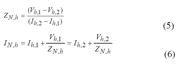
where Vh,1 and Ih,1 are the harmonic voltage and current measurements before the change in the operating condition, and Vh,2 and Ih,2 are the measurements after the change. Note that these equations are complex and moreover the voltage and current magnitudes, their phase angles also should be measured precisely. In the following section, a Norton model is developed for CFLs based on Norton parameters, and the proposed model is compared with the measurement results.
Residential, Commercial and Office loads Norton Equivalent Model
In this section a model for residential, commercial and office loads is developed based on aggregating their corresponding appliances models. To develop the Norton model for each appliance at least two measurements at different operating condition of the supply system are needed. More details about how to achieve the Norton equivalent model parameters using measurement results is described in previous section and [12-14] and 17.
Norton equivalent model parameters consist of ZN and IN for each harmonic order. The Norton equivalent model is developed for each harmonic order separately, and the
complete Norton equivalent model is obtained by combining these models. The Norton model parameters for different residential loads are given in the Table. II.
Table 2. Norton Model Parameters for Residential appliances
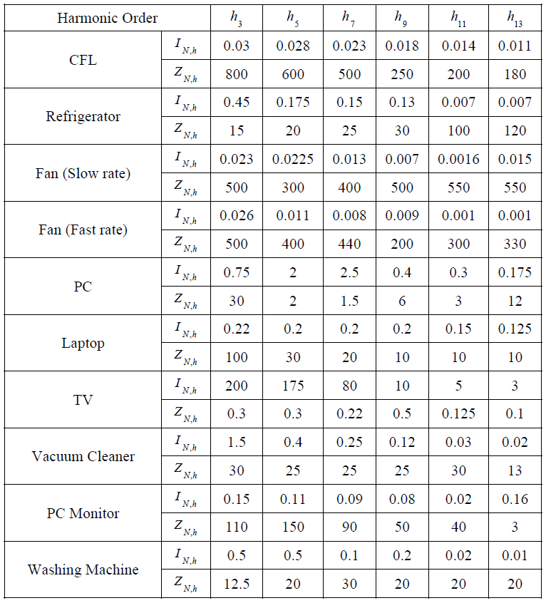
In this work, more than two different operating conditions are considered to obtain better modeling results. The measurement has done at more than two hundred different operating conditions of the supply voltage. The achieved Norton equivalent current and impedances values in different operating conditions converged to a specific value. This convergent make the achieved results more reliable.
After modeling each appliance, residential, commercial and office loads Norton equivalent model will be achieved by aggregating their corresponding appliances Norton equivalent models. In next level a feeder Norton equivalent model will be obtained by aggregating a residential, commercial and office load Norton equivalent models.
Simulation results for a 20 kV Distribution Network
This section analyses the characteristics of a sample distribution network feeder modeled by Norton equivalent technique. This feeder model is obtained based on aggregating the Norton equivalent model of all end user appliances. Obtaining Norton equivalent model of appliances is more described in [14]. A simple schematic for a simple 3 phase balanced distribution network is shown in figure 5 .As figure 5 shows the sample feeder feeds 3 different loads (residential, commercial, office). The total feeder load is equal to the sum of all 3 loads. In this section, a sample office load model and its characteristics are investigated specifically and then characteristics of a feeder composed of residential, commercial, office load models is investigated.
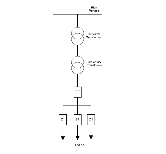
Figure 5: Schematic of a sample 20kV/400V feeder
Using the models for each appliance, an estimation of the power quality of a customer can now be obtained. The assumed office load is supposed to have 2 PCs, 2 CFLs and 2 fans with slow and fast rates. The loads turn on one by one. Figs. 6 and 7 show the rms current and THD of the office load. The point of turning on or off for each appliance is shown in Fig.6.
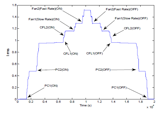
Figure 6: Simulated office load rms current
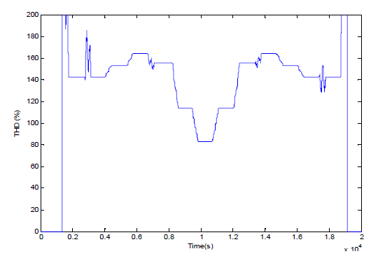
Figure 7: THD trend for simulated office load
The Total Harmonic Distortion (THD) of the office load depends on each appliance THD and its rms value of current. As Figs. 6 and 7 shows the THD decrease as the load current increase.
It is assumed that a 20 KV feeder feeds three different types of residential, commercial and office loads. Each load appliances are as Table.3 shows.
Table 3. Simulated residential, commercial and office loads appliances
| Load type | Appliances |
|---|---|
| Residential | 2 CFLs, Refrigerator, TV, Washing Machine, Vacuum, Iron, Fan |
| Office | 2 PCs, 2CFLs, Laptop, TV, Refrigerator, Printer, Fan |
| Commercial | 2 CFLs, TV, Fan, PC |
The appliances turn on one by one and finally all of the appliances are in on state. Fig. 8 shows the feeder total rms current trend from the starting time up to the time that all of the appliances are turned on.
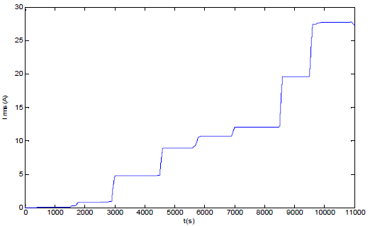
Figure 8: Simulated feeder total current
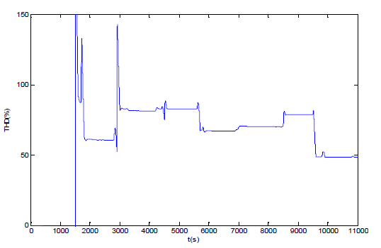
Figure 9: Simulated feeder Total Harmonic Distortion
Figure 9 shows the total harmonic distortion of the feeder current. As this figure shows the THD varies when different appliances turn on. The effect of each appliance on the total feeder THD is dependent on the each appliance THD and its current rms value.
Losses in 20 kV Distribution Networks
In this section losses in transmission lines for the simulated distribution network in section VI are calculated using the equations introduced in section II. Schematic of a sample feeder in figure 5 contains two impedances for the transmission lines (Z1 and Z2). Figure 10 shows the losses due to Z1 impedance for an office load and figure 11 shows losses due to Z2 impedance that three feeder loads current flow through this impedance. As this figures show the loss values increase when the loads turn on and accordingly the lines current increases. The peak value of loss in achieved when all the appliances are turned on. Z1 and Z2 resistances are considered 1 ohm and inductive impedances are neglected.
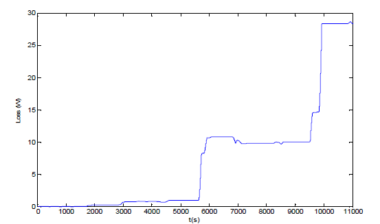
Figure 10: Losses in Z1 impedance for and office load
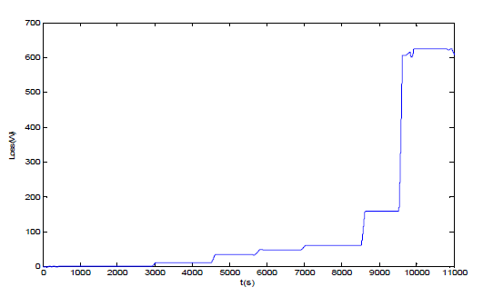
Figure 11: losses in Z2 impedance which feeds three loads
Total loss in Z1 and Z2 impedances for the simulated feeder is shown in figure 12. As Fig.12 shows the loss behavior is similar to the aggregated loads rms current.
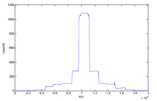
Figure 12: Total losses in Z1 and Z2 impedances
Total amount of losses in this sample feeder reaches to 1100 watt in the maximum stage.
This amount of losses versus the total feeder load is plotted in figure 13.
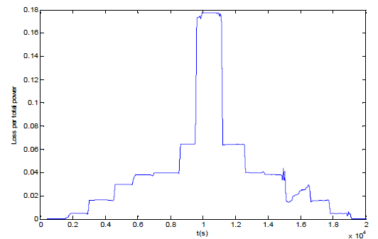
Figure 13: Real power loss versus total feeder real power
The loss in distribution systems is related with the square of the current and this can be seen in the above figures. When the feeder current reaches to its maximum value, the losses value increase in a faster rate and this is because of the quadratic relationship between loss and current.
Losses due to transmission lines impedance for the simulated power network could be increased to 18% of the total feeder power and this amount of loss means a considerable cost for distribution networks that could not be neglected.
Share of nonlinear loads and their harmonics in causing loss of power in distribution
networks could be obtained by the equation 15. According to the figure 9, if the average Total Harmonic Distortion (THD) of the sample power distribution network be considered 50%, then share of the harmonics losses in total losses will be equal to 20% of total loss.
Conclusions
In this paper, a comprehensive investigation has been investigated to determine the effects of harmonic distortions on power system distribution networks. Harmonics due to widespread usage of nonlinear increased recently so that returning to linear load conditions will remain a dream in feature. This work used the Norton equivalent model of different appliances which are obtained by the analyzing the measurement results. Distortion power is defined for common appliances and effect of harmonics on appliances power factor is detailed. The results are reasonably accurate because the Norton equivalent models are pierce and obtained based on the measurements results. Different load type models are achieved by aggregating the Norton equivalent model of individual appliances. A sample feeder is modeled using different residential, commercial and office loads model and losses due to transmission losses are investigated and also share of harmonics in causing extra losses are determined. The results shows that the losses can be increased to 18% percent of the feeder real power and the share of harmonics in these losses is dependent to the total harmonic distortion of the feeder current waveform.
Acknowledgment
The authors of this paper would like to thank Iran Energy Efficiency Organization (IEEOSABA) for their supports in carrying out this research.
References
[1] F. H. Buller and C. A. Woodrow, “Load factor equivalent hours values compared,” Electr. World, Jul. 1928.
[2] H. F. Hoebel, “Cost of electric distribution losses,” Electr. Light and Power, Mar. 1959.
[3] M.W. Gustafson, J. S. Baylor, and S. S. Mulnix, “Equivalent hours loss factor revisited,” IEEE Trans. Power Syst., vol. 3, no. 4, pp. 1502–1507, Nov. 1988.
[4] M.W. Gustafson, “Demand, energy and marginal electric system losses,” IEEE Trans. Power App. Syst., vol. PAS-102, no. 9, pp. 3189–3195, Sep. 1983.
[5] M.W. Gustafson and J. S. Baylor, “Approximating the system losses equation,” IEEE Trans. Power Syst., vol. 4, no. 3, pp. 850–855, Aug. 1989.
[6] D. I. H. Sun, S. Abe, R. R. Shoults, M. S. Chen, P. Eichenberger, and D. Ferris, “Calculation of energy losses in a distribution system,” IEEE Trans. Power App. Syst., vol. PAS-99, no. 4, pp. 1347– 1356, Jul./Aug. 1980.
[7] R. Céspedes, H. Durán, H. Hernández, and A. Rodríguez, “Assessment of electrical energy losses in the Colombian power system,” IEEE Trans. Power App. Syst., vol. PAS-102, no. 11, pp. 3509– 3515, Nov. 1983.
[8] C. S. Chen, M. Y. Cho, and Y.W. Chen, “Development of simplified loss models for distribution system analysis,” IEEE Trans. Power Del., vol. 9, no. 3, pp. 1545–1551, Jul. 1994.
[9] O.M. Mikic, “Variance Based Energy Loss Comptation in LV Distribution Networks”. IEEE Trans. Power Syst., vol. 22, no. 1, pp. 179-187, Feb. 2007.
[10] C.S.Chen, C.H.Lin, “Development of Distribution Feeder Loss Models by Artificial Neural Networks”, IEEE Conference, 2005, Taiwan.
[11]Y.-Y. Hong and Z.-T. Chao, “Development of energy loss formula for distribution systems using FCN algorithm and cluster-wise fuzzy regression,” IEEE Trans. Power Del., vol. 17, no. 3, pp. 794–799, Jul. 2002.
[12]Thunberg, E. and Söder, L., “A Norton Approach to Distribution Network Modeling for Harmonic Studies”, IEEE Trans. Power Delivery, Vol.14, No.1, pp. 272-277, January, 1999.
[13]Thunberg, E. and Söder, L., “On the Performance of a Distribution Network Harmonic Norton Model”, ICHQP 2000, Florida, USA, 01-04 October, 2000.
[14]Abdelkader, S., Abdel-Rahman, M.H., Osman, M.G., “A Norton equivalent model for nonlinear loads”, LESCOPE conference, Halifax, Canada, july, 2001.
[15]Balci, M.E., Ozturk, D., Karacasu, O., Hocaoglu, M.H., “Experimental Verification of Harmonic Load Models”, UPEC conference, Padova, September, 2008.
[16]Jing Yong, Liang Chen, Nassif, A.B., Wilsun Xu, “A Frequency-Domain Model for Compact Fluorescent Lamps”, IEEE Trans. Power Delivery, Vol.25, No.2, pp. 1182-1189, April, 2010. M.J.Ghorbani, H.Mokhtari,”Residential load modeling by Norton Equivalent Model of household loads”, APPEEC 2011, China, 2011.
