Published by
Sean Elphick, Senior Member, IEEE University of Wollongong, elpho@uow.edu.au
Philip Ciufo, Senior Member, IEEE University of Wollongong, ciufo@uow.edu.au
Sarath Perera, Member, IEEE, University of Wollongong, sarath@uow.edu.au
Publication Details
S. Elphick, P. Ciufo & S. Perera, “Laboratory investigation of the input current characteristics of modern domestic appliances for varying supply voltage conditions,” in 14th International Conference on Harmonics and Quality of Power, ICHQP 2010, 2010, pp. 1-7.
Paper link: http://ro.uow.edu.au/engpapers/5519
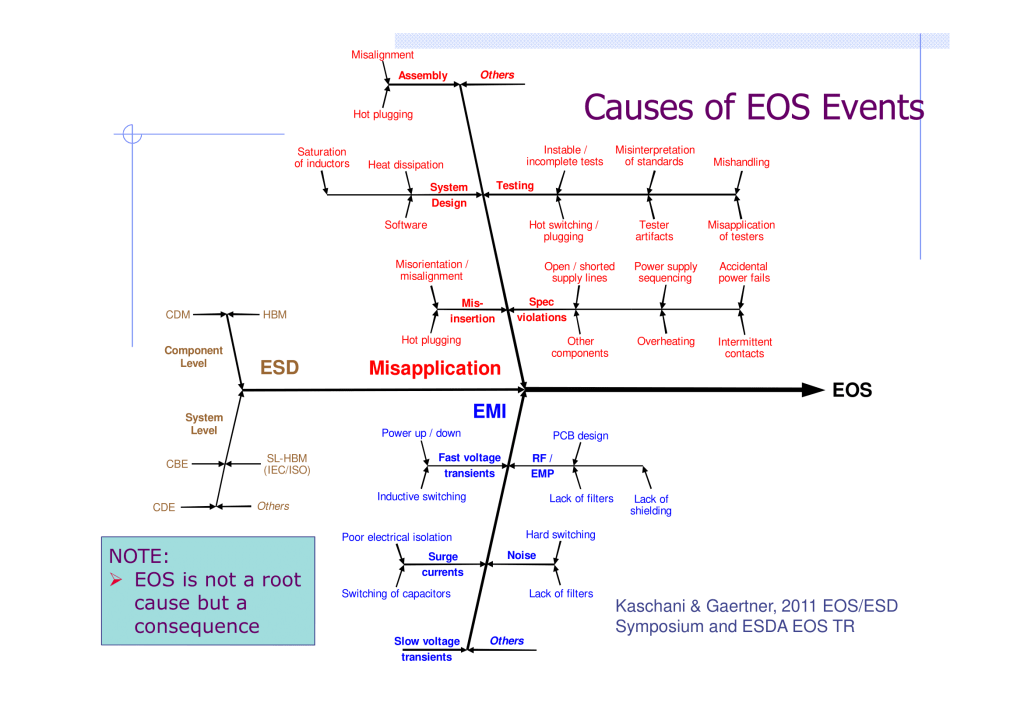
Abstract – The past decade has seen major changes to the appliances which comprise the domestic load. Appliances which may have been considered to be passive loads are now supplied through power electronic front ends. These new loads are known sources of power quality disturbances, predominately harmonic currents. While examinations have been made of the electrical behaviour of first generation electronic appliances, there is little literature dealing with the performance of more modern loads. Understanding the behaviour of modern loads is essential if accurate models of equipment connected to the power system are to be developed. This paper examines the input current characteristics of a number of modern domestic appliances. This includes an analysis under undistorted rated voltage input conditions along with examination of the impact that varying input voltage conditions has on appliance input currents. Characterisation of the appliance input current is achieved through a laboratory testing regime using a programmable power source.
On the whole, it can be noted that many modern appliances have input current performance which is better in terms of harmonic content compared to older appliances with power electronic front ends. With respect to variation of the input voltage, it has been found that harmonic distortion has a larger impact on the input current of appliances than variations in fundamental voltage magnitude.
Index Terms—Harmonics, Input Current, Domestic Appliances, Power Quality
I. INTRODUCTION
The past decade has seen major changes in the individual appliances which comprise the domestic load. Appliances such as whitegoods and lighting which may once have been considered as considered passive loads are now supplied by power electronics. In addition, many electronic appliances have also evolved over time. Examples of evolving technology include air conditioners where direct on-line types have progressed to first generation inverter types and finally to modern inverter driven systems. Another obvious example is televisions where CRT technology has been replaced with plasma and LCD. Recent years have also seen major changes to the lighting load. Many countries have banned the sale of traditional incandescent light globes as a demand reduction strategy. At present, the only viable alternative to the incandescent lamp is the compact fluorescent lamp (CFL).
The modern domestic load also contains a range of appliances which had relatively low penetration levels 10 – 15 years ago. Examples of these appliances include personal computers and DVD players.

Fig. 1. Traditional SMPS Block Diagram [1]
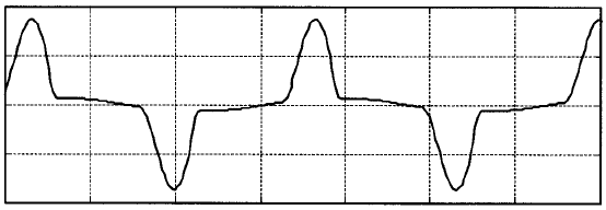
Fig. 2. Traditional SMPS Input Current Waveform [1]
Modern electronic appliances almost universally use a switch-mode power supply (SMPS). These have a number of advantages and the most notable is the ability to operate over a wider range of input voltage magnitudes. The block diagram of a typical SMPS is shown in Fig 1. The characteristic ac side current waveform of a SMPS, when supplied with a sinusoidal input voltage from a strong supply, is shown in Fig 2.
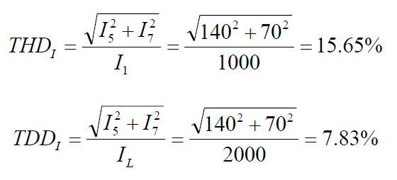
The current harmonic spectrum for the waveform in Fig. 2 is shown in Fig 3. The harmonic spectrum is dominated by high magnitudes of low order odd harmonics such as 3rd, 5th and 7th which decay rapidly with frequency. 3rd harmonic is always the dominant harmonic order.

Fig. 3. Traditional SMPS Input Current Harmonic Spectrum [1]
Studies presented in [2] and [3] describe the impact of changes in input voltage supply characteristics on the input current characteristics of appliances supplied by SMPS. However, these studies are now quite dated. While the basic SMPS topology shown in Fig 1 has been in existence for many years there is evidence to suggest that developments have been made to the design of appliances supplied by SMPS. These changes have been made in order to improve the ac side harmonic current performance of the appliances [4].
The study presented in [5] is more recent. However, it is limited to investigating the impact of ac supply voltage waveform distortion levels on ac side supply current THD levels. The work presented in this paper complements and expands on the work presented in [5]. An examination of the impact of the variations in both the magnitude and distortion level of the input voltage on the input current characteristics of a number of modern domestic electronic appliances is made. A range of input current parameters are studied including RMS current, displacement power factor, total harmonic current and individual harmonic current orders. The investigations have been performed using a 30 kVA programmable source combined with power quality measurement instrumentation. The programmable source used has output voltage distortion levels of less than 1% THD when supplying sinusoidal voltage waveforms. The power quality instrumentation used is a Hioki 3196 power quality analyser which is a IEC61000-4-30 [6] Class A compliant instrument.
II. APPLIANCES TESTED
A range of common domestic appliances has been tested. Selection of the appliances to be tested was based on a combination of appliance penetration levels as well as power usage magnitude. The appliances tested are likely to be found in a majority of homes or represent appliances which have large power demand and as such may have larger impact on the electricity distribution network. Small appliances such as mobile phone chargers have not been included in testing. The appliances tested are:
- 15 W CFL Lighting. Three different CFLs were examined.
- Televisions (TVs). Three technologies; CRT, plasma and LCD. The CRT is a 51cm model while the plasma and LCD are 32 inch models.
- 3.3 kW split system Inverter Air Conditioner.
- 2.4 GHz Personal Computer (PC).
- 17 inch LCD Computer Monitor.
- DVD player.
III. TEST SCHEDULES
Each appliance was subjected to a range of tests to determine performance under varying input voltage conditions which were selected based on levels that are likely to be experienced on Australian low voltage (230V/400V) electricity distribution networks. Each appliance was subjected to five distinct tests. Each test involved application of different input voltage magnitudes or waveform distortion levels. The first three tests were designed to examine the operation at undistorted voltage magnitudes representing the range of operating conditions encountered on a distribution network under normal conditions. The second two tests were designed to assess the impact that harmonic distortion of the input voltage waveform had on appliance input current. Two test waveforms have been developed to facilitate this. The levels of harmonic distortion on the two harmonic test waveforms were selected to represent feasible harmonic magnitudes and phase angles likely to be encountered on Australian low voltage networks [7]. Each of the harmonic test waveforms applied to the appliances have a fundamental voltage of 230 V.
Table 1 details the specific magnitudes used for each harmonic test waveform while Fig 4 shows the actual waveforms. The characteristics of the test waveforms were established using data from the Australian Long Term Power Quality Survey [7] as well as a number of field measurements. These measurements indicate that voltage THD levels will be less than 3.67% at 95% of sites with the dominant harmonic order being the 5th. Other harmonic orders which make significant contributions are low order such as 3rd and 7th. Higher order harmonics have been noted to be generally small in magnitude. Other field studies have shown that most supply voltage waveforms exhibit a flat top characteristic. This allows basic determination of the phase angle of the harmonic voltages. Such flattening can be shown to be caused by a 3rd harmonic component which has a phase angle of close to 0 degrees with respect to the fundamental and a 5th harmonic component which has a phase angle close to 180 degrees with respect to the fundamental. Field monitoring confirms these observations. Field monitoring also shows 7th harmonic phase angles close to 50 degrees. Harmonic test waveforms 1 and 2 have THD levels of 3.3% and 4.7% respectively.
TABLE 1: HARMONIC TEST WAVEFORM DETAILS


Fig. 4. Harmonic Test Waveforms
IV. CHARACTERISTICS AT NOMINAL VOLTAGE
In this section of the paper, the performance of each device is examined when supplied at 230 V (Australian LV nominal voltage) with no additional waveform distortion. The following key aspects are examined for each device:
- Input Current Waveform
- Displacement Power Factor (DPF)
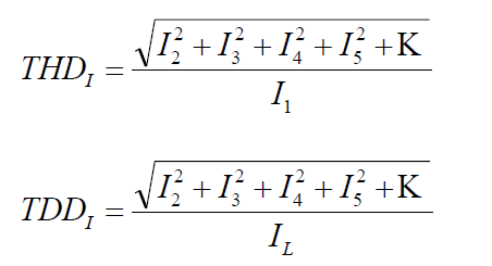
- Current Total Harmonic Distortion (ITHD)
- Harmonic Current Spectrum
A. CFLs
The CFL is a well known non-linear load [8] and [9]. In [8] it is shown that there can be significant differences in the performance of CFLs depending on the front end input circuitry. With a view to examine the differences in CFL performance, three types are examined here. These CFLs are representative of the range of lamps available. Two of the types are widely available models. The third type is known as a high power factor CFL and contains components designed to improve the harmonic content of the input current, that is, to correct the true power factor. Fig 5 shows the input current waveforms for the three CFLs tested. It can be seen that there is significant variation in the input current waveforms across the three CFL samples. The high power factor CFL, i.e. sample 3 in Fig. 5, is seen to have a more sinusoidal input current than the other two CFLs that are characterised by extremely peaky input current waveforms. It is also of note that the CFL input current waveform is quite different to that of the simple SMPS current waveform as shown in Fig 1.

Fig. 5. CFL Input Current Waveforms
The waveforms shown in Fig 5 for CFL samples 1 and 2 indicate that their input current waveforms are rich in harmonics. The harmonic spectrum for each of the 3 CFLs tested is shown in Fig 6. Only odd order harmonics are shown as even order harmonic components were found to be negligible.

Fig. 6. CFL Input Current Harmonic Spectra
Fig 6 shows that CFL Samples 1 and 2 are characterised by relatively large low order harmonic components. Of particular interest is the current harmonic spectrum of CFL sample 1 which shows significant harmonic current harmonic components up to the 49th (the limit of measurement). This is highly atypical of the harmonic spectra of equipment supplied by a SMPS and indicates that some CFL types may have unexpected harmonic behaviour not exhibited by other domestic loads.
B. Televisions (TVs)
Television (TV) technology has undergone significant changes over the past ten years with the traditional CRT TV making way for newer technologies such as plasma and LCD. These new technologies have provided the capability for much larger screen sizes but at the expense of higher power demand. Three TV technologies, i.e. CRT, plasma and LCD have been examined. The input current waveforms for these devices are shown in Fig 7.

Fig. 7. TV Input Current Waveform
Studies such as [10] have shown that TV load can be attributed to significant harmonic levels on distribution networks. With the increased power rating of modern TVs it has been assumed that harmonic current levels would also be higher than seen for CRT TVs. However, the waveforms shown in Fig 7 indicate that this may not be the case. The waveforms for the plasma and LCD TVs are considerably more sinusoidal than that of the CRT TV. Fig 8, which shows the harmonic spectra of the TVs tested, clearly indicates that the newer TV technologies (Plasma and LCD) lead to considerably smaller harmonic current components than the CRT TV in spite of their higher power demand.

Fig. 8. TV Input Current Harmonic Spectra
C. Inverter Air Conditioner
First generation inverter air conditioners have been observed to be highly non-linear loads. When these air conditioners were introduced, there were serious concerns regarding the impact of these devices on distribution network harmonic levels [11]. First generation inverter air conditioners displayed current waveforms and harmonic components typical of a SMPS. However, the air conditioner power demand is likely to be much greater than that of any other electronic device in the domestic load and hence leading to concerns on large current harmonic components.
A 3.3 kW inverter air conditioner from a large international manufacturer has been examined. The nearly sinusoidal input current waveform for this device is shown in Fig 9. This is surprising given the peaky and harmonic rich waveforms of older style inverter air conditioners. This indicates that manufacturers of modern air conditioners have developed input circuitry which mitigates the input current distortion of first generation air conditioners.

Fig. 9. Inverter Air Conditioner Input Current Waveform
D. Personal Computer (PC)
Penetration levels of personal computers (PCs) in domestic residences has grown from negligible levels in 1994 [12] to 87% in 2008 [13]. The PC examined here is a desktop Pentium 4, 2.4 GHz Intel processor model. Fig 10 shows the input current waveform for the PC. The waveform is characteristic of a basic SMPS. Fig 11 which shows the current harmonic spectrum of the PC for odd order harmonics also displays harmonic components characteristics of the traditional SMPS. It can be seen that significant levels of harmonic current are observed for harmonic orders up to the 23rd, however, unlike the CFL, harmonic components are negligible beyond this point.

Fig. 10. PC Input Current Waveform

Fig. 11. PC Input Current Harmonic Spectrum
Monitors for PCs are now almost exclusively LCD types as opposed to CRT. The monitor tested here is a 17 inch model manufactured by an international supplier. The input current waveform and harmonic spectrum as shown in Figs 12 and 13 respectively indicate that the LCD monitor has characteristics similar to the personal computer and characteristics of a simple SMPS.
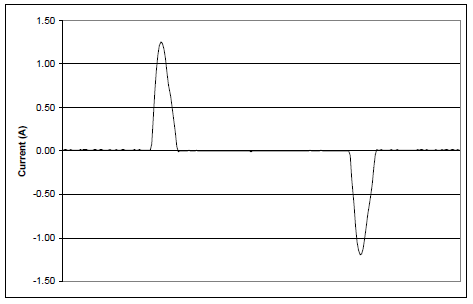
Fig. 12. 17 inch LCD Monitor Input Current Waveform

Fig. 13. LCD Monitor Input Current Harmonic Spectrum
F. DVD Player
The DVD player tested showed an input current waveform and input current harmonic spectrum similar to that observed for the LCD monitor and characteristic of a SMPS. As the results are similar to those seen for the personal computer and LCD monitor, graphs of input current waveform and harmonic spectrum are not shown here.
V. IMPACT OF VARIATION OF INPUT VOLTAGE
The impact of variations in the input voltage on the input currents of each of the appliances tested is examined in this section. Understanding the implications of variation to the input current of appliance due to changes in the input voltage is essential for complete understanding of the manner in which appliances may impact on the electricity distribution system. An accurate understanding of appliance behaviour under changing input voltage conditions is also essential if accurate appliance models are to be developed for simulation.
Four tests have been designed to assess the impact of variations in input voltage on appliance input current behaviour. The first two tests examine appliance behaviour at the upper and lower limits of the Australian low voltage range. The first of these tests involved supplying the appliances at 253 V RMS which is at the upper limit of the range and the second involved supplying the appliances with 207 V RMS which is at the lower limit of the range. The remaining tests involved supplying the appliances with distorted input voltages.
In order to easily identify the difference between values obtained for each test and the results obtained using the undistorted nominal value (230 V RMS), the data in each table in this section of the paper is expressed as a percentage of the values obtained when the nominal voltage was applied. For example, a value of 100% means that the value obtained for the test was equal to the value obtained when the appliance was supplied with an undistiorted voltage of 230V RMS.
A. Impact of Varying Input Voltage Magnitude
Table 2 shows the results of the first test (supply at 253 V RMS) for RMS current (I RMS), displacement power factor (DPF), fundamental current (I Fund) and the total harmonic current.
TABLE 2: VARIATION IN I RMS, DPF, I FUND AND TOTAL HARMONIC CURRENT -253 V RMS INPUT VOLTAGE
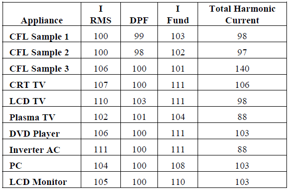
Table 3 shows the same data as in Table 2 for the second voltage magnitude test (supply at 207 V RMS).
TABLE 3: VARIATION IN I RMS, DPF, I FUND AND TOTAL HARMONIC – 207 V RMS INPUT VOLTAGE
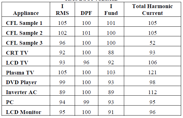
The data in Tables 2 and 3 indicate that the behaviour of the RMS current, displacement power factor and fundamental current is relatively insensitive to changes in the supply voltage magnitude. Results for total harmonic current are more varied. CFL Sample 3, the plasma TV and the inverter air conditioner show considerable variation in total harmonic current for one or both of the voltage magnitude tests. It is notable that the CFL, plasma TV and air conditioner appear to have electronics on the input which aim to mitigate current waveform distortion. It may be postulated that these circuits are more sensitive to changes in input supply voltage than more simple devices such as the SMPS of the PC.
An examination has also been made of the impact of varying the input voltage magnitude on selected individual harmonic current orders. For the purposes of this study, the harmonic orders investigated are 3rd, 5th and 7th which are the dominant harmonic orders which prevail in low voltage networks. The results of this investigation are shown in Table 4.
TABLE 4: VARIATION IN INDIVIDUAL CURRENT HARMONIC ORDERS – 253 AND 207 V RMS INPUT VOLTAGE
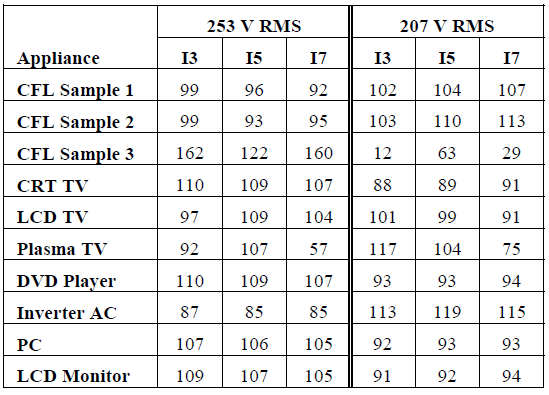
Table 4 shows that there is considerably more variation in individual harmonic current components than was observed for the current parameters shown in Table 4. Those appliances which showed the greatest variation in total harmonic current are also seen to have the most extreme variation in individual harmonic current components. The foremost of these is CFL Sample 3 where low order current harmonic behaviour shows extreme sensitivity to the input voltage magnitude.
B. Impact of Varying Input Voltage Distortion Level
Two tests were performed to asses the impact of distorted input voltages on the input current of the appliances. These tests involved the application of the two harmonic test waveforms described in Section III. The fundamental voltage applied for both waveforms was 230 V. Tables 5 and 6 illustrate the values of a range of basic parameters for the 2 voltage distortion tests.
TABLE 5: VARIATION IN I RMS, DPF, I FUND AND TOTAL HARMONIC CURRENT – HARMONIC TEST WAVEFORM 1

Table 5 indicates that there is little variation in the displacement power factor and fundamental current when the appliances are supplied with harmonic test waveform 1. However, there is considerable variation seen for RMS current and total harmonic current. Further, the variations seen here are much greater than those observed in the previous section where input voltage magnitude was varied. This indicates that appliance behaviour is more sensitive to changes in input voltage distortion as opposed to changes in input voltage magnitude.
TABLE 6: VARIATION IN I RMS, DPF, I FUND AND TOTAL HARMONIC CURRENT – HARMONIC TEST WAVEFORM 2

Similar results are observed in Table 6 to those seen in Table 5. Variation in displacement power factor and fundamental current is modest, however, variations in RMS current and total harmonic current are significant.
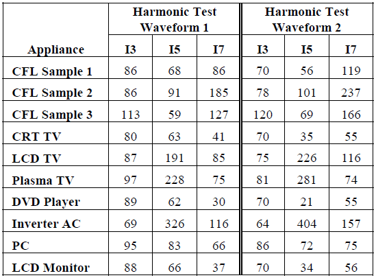
Table 7 shows the variation in low order individual harmonic current orders when harmonic test waveforms 1 and 2 are used to supply the appliances. It can be seen that there is considerable variation in all harmonic orders for most appliances.
TABLE 7: VARIATION IN INDIVIDUAL CURRENT HARMONIC ORDERS – HARMONIC TEST WAVEFORM1 AND 2
VI. CONCLUSIONS
This paper has presented typical supply current waveforms for a number of modern domestic appliances. It has also examined the impact of variations in supply voltage have on the input current behaviour of a range of modern domestic appliances. In practice it is unlikely that appliances connected to electricity networks will be supplied at undistorted nominal voltage levels. Understanding how appliances behave when subjected to input voltages which are realistic is essential for understanding the behaviour of devices connected to the electricity network for the purposes of network planning, modelling and analysis.
The investigations undertaken in this paper indicate that the basic input current characteristics of the appliances tested are relatively insensitive to changes in the magnitude of an undistorted supply voltage. Variation of low order individual harmonics between the nominal voltage case and a raised or lowered voltage case were found to be significantly larger than basic quantities such as RMS current or fundamental current. However, for most appliances, the variation was relatively small.
Investigations completed using distorted input voltages indicated that the input current characteristics of most devices were highly sensitive to distortion in the input voltage. Harmonic distortion on the input voltage was found to have a much greater impact on the input current of each appliance than was the case for changes in undistorted supply voltage magnitude.
VII. REFERENCES
[1] Roger C. Dugan, Mark F. McGranaghan, Surya Santoso, H. Wayne Beaty, “Electrical Power Systems Quality”, Second Ed, McGraw-Hill, NY, 2003
[2] A. Mansoor, W. M. Grady, R. S. Thallam, M. T. Doyle, S. D. Krein, M. J. Samotyj, “Effect of Supply Voltage Harmonics on the Input Current of Single-Phase Diode Bridge Rectifier Loads”, IEEE Transactions on Power Delivery, Vol. 10, No. 3, July 1995, Page(s): 1416 – 1422
[3] Michael J. Ouellette, Réjean Arseneau, “The Effects of Undervoltage on the Performance of Compact Fluorescent Systems”, IEEE Industry Applications Society Annual Meeting, 4 – 9 Oct 1992, Vol.2 Page(s):1872 – 1879
[4] Sean Elphick, Phil Ciufo, Sarath Perera, “Supply Current Characteristics of Modern Domestic Loads”, Proc. AUPEC 09, 27th – 30th September 2009, Adelaide, Australia, Paper PP086
[5] Matthew Rylander, W. Mack Grady, and Martin Narendorf, Jr., “Experimental Apparatus, Testing Results, and Interpretation of the Impact of Voltage Distortion on the Current Distortion of Typical Single-Phase Loads”, IEEE Transactions on Power Delivery, Vol. 24, No. 2, April 2009, Page(s): 844 – 851
[6] IEC61000-4-30, “Electromagnetic Compatibility (EMC) –Part 4-30: Testing and Measurement Techniques – Power Quality Measurement Methods, IEC Standard, 2003.
[7] Australian Long Term Power Quality Survey Reports, Confidential reports to participants, 2002 – 2010
[8] Neville R. Watson, Tas Scott and Stephen Hirsch, “Compact Fluorescent Lamps (CFL) – Implications for Distribution Networks”, 83rd Annual EESA Conference and Exhibition, Electricity 2007, Melbourne, Australia, 15 – 17 Aug 2007
[9] M. H. Sadek, A. A. Abbas, M. A. El-Sharkawy, Hussein M. Mashaly, “Impact of Using Compact Fluorescent Lamps on Power Quality”, ICEEC ’04, International Conference on Electrical, Electronic and Computer Engineering, 5-7 Sept. 2004 Page(s):941 – 946
[10] N. Browne, S. Perera, P. F. Ribeiro, “Harmonic Levels and Television Events”, 2007 IEEE Power Engineering Society General Meeting, 24-28 June 2007, Page(s):1 – 6
[11] D. Essah, E. Feiste, R. O’Connell, R. G. Hoft, G. Brownfield, “Harmonic Effects of Variable Speed Air Conditioners on a Single-Phase Lateral and on the Distribution Feeders in a Typical Power System I”, 9th Annual Applied Power Electronic Conference and Exposition, APEC’94, 13-17 Feb, 1994, vol.2, Page(s):622 – 627
[12] “Australian Social Trends”, Australian Bureau of Statistics, Document 4102.0, 2006, Page(s) 191 – 195
[13] “Energy Use in the Australian Residential Sector 1986 – 2020”, Australian Government Department of the Environment, Water, Heritage and the Arts, 2008
VIII. BIOGRAPHIES

Sean Elphick graduated from the University of Wollongong with a BE (Elec)(Hons) degree in 2002. He commenced employment with the Integral Energy Power Quality Centre in 2003. Initially employed to work on a Strategic Partnerships with Industry – Research and Training Scheme (SPIRT) project dealing with power quality monitoring and reporting techniques. His current activities include delivery of the Long Term National Power Quality Survey, a first of its type in Australia as well as various other power quality related research and consulting projects.

Philip Ciufo (M’1990, SM’2007) graduated from the University of Wollongong with a B.E. (Hons) in Electrical Engineering in 1990 whilst also completing an Industry Cadetship. In 1991 he joined the University as Research Associate where he worked on several research projects and provided engineering support to many of the research programs within the School of Electrical Computer and Telecommunications Engineering. He obtained an M.E. (Hons) in Electrical Engineering 1993. He joined the academic staff of the University after completing his Ph.D. in 2002. The title of his thesis was “Magnetic Modelling and Sensorless Control of the Synchronous Reluctance Machine”. Dr Ciufo has had various stints in industry as an Electrical Engineer and returned to academia in 2007. His research interests include Modelling and Analysis of Power Distribution Systems, Distribution Automation, Modelling and Analysis of ac Machines, Power System Harmonics and Power System Reliability.

Sarath Perera (M’1995) received the B.Sc.(Eng.) degree in power from the University of Moratuwa, Sri Lanka, in 1974, the M.Eng.Sc. degree from the University of New South Wales in 1978, and the Ph.D. degree from the University of Wollongong in 1988. He was a Lecturer for twelve years with the University of Moratuwa. Currently he is an Associate Professor with the University of Wollongong and is the Technical Director of the Integral Energy Power Quality and Reliability Centre. His research interests are in power quality.