Published by Jürgen Blum, Product Manager, Power Quality, A. Eberle GmbH & Co. KG
In the first part of the measurement campaign of 2016, various electric vehicles were evaluated in terms of their charging behavior and their loading effects on the power grid. The evaluation covered from DC up to the 50th harmonic or supraharmonics up to 20 kHz. As some electric vehicles use a chopper frequency much higher than 20 kHz, another measurement campaign was started at the University of Applied Sciences Bingen in September 2017 to measure the emissions ranging up to 150 kHz. In addition, the mutual interference between the different vehicles and between the electric vehicle and a solar inverter was investigated at the University of Applied Sciences Bingen.
Basis of the evaluation of the loading effects
The IEC 61851-21-1 standard (Electric vehicle on-board charger EMC requirements for conductive connection to AC/DC supply) will apply to electric vehicles in the future. This standard has already received the status of FDIS and will be published shortly.
At this time, the limits for current harmonics as given by IEC 61000-3-2 (Class A) up to 16 A and IEC 61000-3-12 (asymmetrical devices, Rsce = 33) for 16 A up to 75 A apply to electric vehicles. These same compatibility levels are also used in IEC 61851-21-1. There are limits up to the 40th current harmonic (2 kHz) and compatibility levels from 150 kHz to 30 MHz. There are no limits now on the emitted interference from electric vehicles in the frequency range from 2.5 kHz to 150 kHz. This range is also not regulated for the public power grid using compatibility levels. However, there are efforts underway now in the standards committee aimed at closing this gap as quickly as possible using compatibility levels.
There are many examples today of the mutual interference between different electronic devices. For example, the frequency converter of a CNC machine emits an interference level > 2.5 kHz into the power grid and a kitchen appliance malfunctions, or a solar inverter can automatically switch touch-dimmer lamps on and off. Who is responsible for this problem?
Is the kitchen appliance improperly equipped for interference resistance or is the CNC machine causing too large an interference level in the power grid at its connection? There can only be a fair regulation with the forthcoming limits for this frequency range. The interference can be remedied at both ends. Install a power filter on the device experiencing interference or reduce the emitted interference at its origin. Different customers always ask the question, „Who has to pay for it?“
The current draft of IEC 61000-2-2 (Compatibility levels for the public power grid) defined limits for the following ranges:
| Frequency range (kHz) at 50 Hz | Compatibility level (%) |
|---|---|
| 2 kHz to 3 kHz | 1,4 % |
| 3 kHz to 9 kHz | 1,4 to 0,65 % Logarithmic drop-off with logarithmically increasing frequency |
| Frequency range (kHz) | Compatibility level (dBμV) |
|---|---|
| 9 kHz to 30 kHz | 129 to 122 dBμV Linear drop-off with the logarithm of the frequency from 9 to 30 kHz |
The range of 30 kHz to 150 kHz is being prepared; compatibility levels are being added in real time.
In the standard, intentional emissions, for example, PLC signals for communication, are distinguished from nonintentional emissions.
Power utilities make use of a power line signal in the frequency range up to 148 kHz for signal transmission over the power grid. So that this signal can be detected unambiguously by the receiver, there must be a gap between the nonintentional emission from the power electronics, such as that caused by electric vehicles, and the PLC signal. Consequently, two limit curves are given in the standard.
| Voltage (mV) | dBμV |
|---|---|
| 1000 mV | 120 dB |
| 100 mV | 100 dB |
| 10 mV | 80 dB |
Measuring technology
Today, there are not many power quality measurement devices for permanent, uninterrupted monitoring of frequencies from DC to 150 kHz. This comes from the fact that there are no specifications as to how to evaluate in the future standard-compliant levels > 2.5 kHz to 150 kHz.
The measuring procedure for the frequency range from 2 kHz to 9 kHz is described in the standard for harmonics, IEC 61000- 4-7 in the informative Annex B. In this case, a grouping procedure for frequency bands of 200 Hz is used.
For the range > 9 kHz to 150 kHz, there is a suggestion in the Annex to IEC 61000-4-30, Ed. 3. Here, a grouping procedure for bands of 2 kHz is suggested. The final measuring procedure will only be specified in a few years in the future Edition 4 of IEC 61000-4-30. The frequency bands of 200 Hz or 2 kHz are under discussion. While a 200 Hz frequency band provides greater resolution in the spectrum, 10 times the quantity of data is measured than with a 2 kHz frequency band. Because of this, each procedure has advantages and disadvantages.
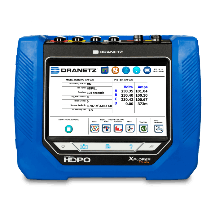
The PQ Box 300 from the A. Eberle company was used for the measurement campaign at the University of Applied Sciences Bingen. The power quality network analyzer measures frequencies from DC to 170 kHz with high accuracy. The grouping procedure of the measurement device can be configured for either 200 Hz or 2 kHz frequency bands. In this way, the different measurement results coming from the different grouping procedures can be verified.
For charging the various electric vehicles, a charging station with a type 2 charging plug and various 32 A CEE outlets and single-phase outlets was available.
The charging station was connected to the power grid of the University and uses a 25 mm² cable. The short-circuit performance at the charging station is about 2.5 MVA. A single phase 5 kW inverter is connected at a distance of about 10 m. The distance, that is the length of the cable connections, between the electric vehicles connected to the charging station, was usually 10 m, 2 times a standard charging cable of 5 m.
Measurement results
The following electric vehicles were evaluated:
Renault Zoe, Nissan Leaf, BMW i3, Audi e-tron, VW Golf GTE, Ford Focus e-lectric, Mitsubishi Outlander and the Tesla Model 90D.
Measurements were performed in the following configurations:
- The electric vehicle alone to the power grid
- The electric vehicle in parallel with other electric vehicles
- The electric vehicle in parallel with the solar inverter of the University
The chopper frequencies of the vehicles measured were between 8 kHz and a maximum of 50 kHz for the different manufacturers.
In addition, there were large differences in the levels of the switching frequencies for the various vehicles. These were between 2 volts for vehicles with poor filtering and high interference levels as well as values that were undetectable by measurement in vehicles with an extremely low interference level.
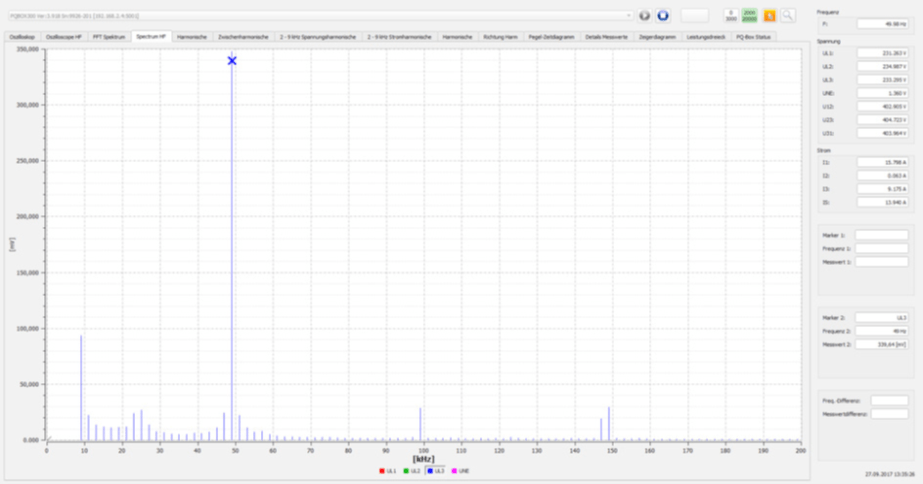
Fig. 1: Electric vehicle with a 50 kHz chopper frequency; shown with 2 kHz frequency bands
Fig. 1 depicts the voltage using 2 kHz frequency bands up to 170 kHz A chopper frequency of 50 kHz can clearly be seen on an electric vehicle. The harmonics of 100 kHz (2 x 50 kHz) and 150 kHz (3 x 50 kHz) can also be seen.
The measuring procedure must be clearly defined for future evaluations of the compatibility levels of electric vehicles or other power electronics connected to the power grid. For example, if you compare the measurement results of 5 Hz, 200 Hz or 2 kHz frequency bands with one another, it is obvious that the results for level can differ substantially from one another. A broader frequency band of 2 kHz usually yields a larger measurement result than a narrow 200 Hz band for the same interference signal in the power grid (see Fig. 1 and Fig. 2 for comparison). With a broad frequency band, several spectral lines are quadratically added to one measurement value.
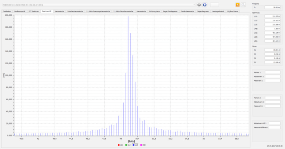
Fig. 2: Electric vehicle with a 50 kHz chopper frequency; shown using 200 Hz frequency bands
Fig. 2 shows the identical 50 kHz loading effect as the electric vehicle shown in Fig. 1. In each case, only the grouping procedure was switched in the measurement device from 2 kHz bands to 200 Hz bands.
Mutual interference between electric vehicles
During the measurement campaign, different electric vehicles were also charged in parallel to be able to evaluate the mutual interference between the vehicles.
Connection configuration 1: Electric vehicle No. 1 on the power grid alone
The vehicle is charged using one phase (C). In the figure, you can see the voltages A, B, C and the charging current C for the electric vehicle. No pronounced loading effects can be seen on the current. The switching frequency of this vehicle was 50 kHz.

Fig. 3: Electric vehicle No. 1 connected to the outlet alone
Connection configuration 2: Electric vehicle No. 1 is connected to the outlet and electric vehicle No. 2 in connected in parallel to the charging station using the type 2 plug.
The following Fig. 4 shows a clear change in the current consumption of electric vehicle No. 1 due to the loading effects from electric vehicle No. 2. The RMS value is virtually unchanged but there are large peaks in the charging current at the switching frequency of vehicle No. 2.
Vehicle No. 1 is connected to the power grid acting as an interference sink for the supraharmonics of the adjacent vehicle. In this example, a 10 kHz switching frequency can barely be seen in the voltage but is very pronounced in the current.
There are reports from practical use that sporadic interruptions in charging may occur if various different electric vehicles are charged in parallel.
Fig. 4: Electric vehicles No. 1 and No. 2 connected in parallel to the charging station and the outlet
Additional striking features
Almost all vehicles using single-phase charging used phase A. Only one vehicle used phase C for single-phase charging. This can later become a real problem by overloading phase A in the power grid with a greater number of vehicles in a supply power grid.
In addition, a large power grid imbalance occurs at the stub-end feeders. Even some vehicles, which were charged in the beginning using 3 phases, switched automatically toward the end to single-phase charging. This charging then usually used phase A.
In the engineering guides for connecting customer systems to the low-voltage grid of power utilities (VDE-AR 4100), the maximum connection power for single-phase loads is limited to <= 4.6 kVA. Electrical loads or generation systems 4.6 kVA must be connected using three phases. As a result, some of the electric vehicles from the measurement campaign may not be operated at a maximum connection power of up to 7.2 kVA.
Example: Electric vehicle with a single-phase charging current of 30 A on phase A
Fig. 5: Electric vehicle, single-phase charging at 6.9 kVA
Audible disturbance effects and summation with electric vehicles having the same switching frequency
One electric vehicle with a pronounced switching frequency of 10 kHz was clearly audible for the human ear in this frequency range during the charging process. Two vehicles of the same type were charged in parallel. The summation of the switching frequency in the power grid as well as the audible disturbance were evaluated.
As the switching frequency of both vehicles is not precisely 10 kHz but rather varies around 10 kHz, the level of the power grid loading effect fluctuates between a minimum of 1 V and a maximum of 2 V. One vehicle alone with a constant loading effect was about 1.4 V. As a result, both switching frequencies could add over time or also partially offset depending on the instantaneous phase difference of the frequencies.
If you stood exactly in the middle between the two vehicles during charging, you could hear the volume of the perceptible whistle change. In one case from practice, some vehicles from the same manufacturer caused a disturbance in an office building adjacent to several charging stations. This disturbance was so loud that the windows on the lower floor of the building could no longer be opened during office hours (reason: noise pollution).

Fig. 6: Chopper frequency of 2 electric vehicles of the same type and the photovoltaic inverter
Fig. 6 shows the 10 kHz chopper frequency of two electric vehicles of the same type and the 16 kHz of the solar power plant at the University of Applied Sciences Bingen. This amplitude of the switching frequency for both electric vehicles fluctuated in the measurement values between 1 V and 2 V at a frequency of about 0.5 Hz.
Mutual interference between electric vehicles and the solar inverter
The following figure shows the initial power grid load with an inverter and a solar power plant. You can see the chopper frequency of 16 kHz and its harmonics at 32 kHz, 48 kHz, and so on.

Fig. 7: Chopper frequency of the photovoltaic inverter
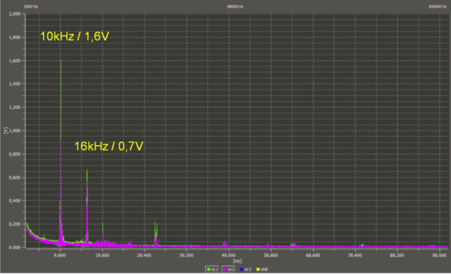
Fig. 8: Chopper frequency of the photovoltaic inverter and one electric vehicle
Now, an electric vehicle is connected to the charging station. You can now clearly see the 10 kHz switching frequency of the vehicle with 1.6 V in the power grid. The 16 kHz level of the solar inverter was, however, reduced by 50% from 1.4 V to 0.7 V.
Summary
Electric vehicles and modern power electronics may generate loading effects on the power grid far above 2.5 kHz. In the future, there will be compatibility levels for the public power grid for these frequencies. The measuring procedure for this is not been defined at this time. The PQ Box 300 from A. Eberle measures the range up to 170 kHz as a continuous measuring task. The measurement device can be set to frequency bands of 200 Hz or 2 kHz. This feature makes it ready for future changes to the standards. In addition, it is possible to select a different measuring procedure than for the parallel online measurement for recording.
Example: Continuous measurement of the 2 kHz bands and, in parallel, 200 Hz bands for online monitoring of a load. The network analyzer uses a continuous measuring procedure as the basis for calculating the FFT analysis.