Published by Carelabs (Carelabz), Website: carelabz.com
Image: Carelabz
Infrared Scanning of electrical installations falls under classification of Predictive Maintenance Fault Finding. The value is that we are now able to predict an electrical fault before the element fails completely.
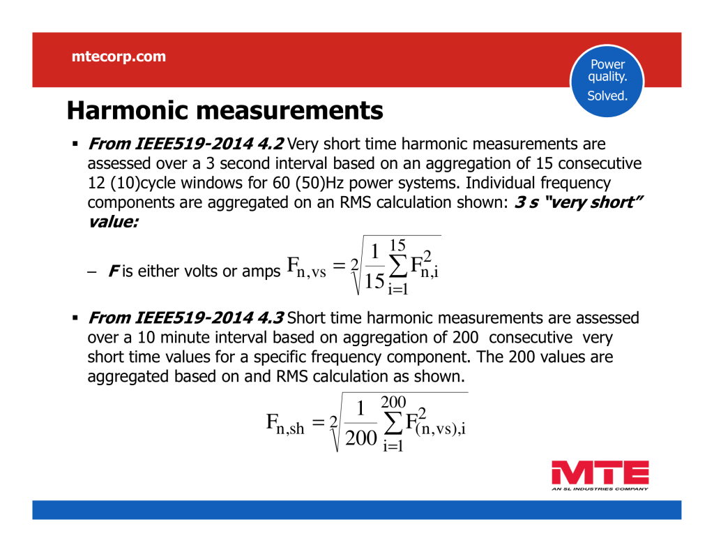
We are able to get this due to the heat build-up of any electrical element under stress and predict that it will fail while it is still functional and appears normal to the naked eye or any other test equipment. The heat signature identified with the use of an Infrared camera. The pictures are then analysed and put into an easy-to-follow report so that they can rectify before a breakdown occurs, preventing loss of production due to unplanned down time.
Unexpected breakdowns in electrical supply can inconvenient and costly. Infrared electrical thermography is a useful tool that can recognize stressed elements of your electrical installation before they break down or cause a fire. This gives you the opportunity to solve the problem as part of planned maintenance before it causes a serious problem.
Another result of failed or stressed electrical elements is the risk of fire; in fact the risk is more real than commonly realise. It is in this vein that insurance companies are increasingly calling for infrared electrical thermography surveys as a valuable risk assessment aid.
In the past this service was only available to very large companies and mining houses due to the cost determinant, but as with everything there have been massive advancements in the last few years and Thermo Scanning has now become a very profitable tool in the small to medium size business world.
Maintenance includes vibration analysis on machines, audio, ultrasonic and infrared thermography inspection on electrical systems. Thermography used to recognize equipment hot spots. This task is typically carried out using temperature sensing instruments like thermocouple sensors or other forms of thermometers. Limitation of this analysis is that this kind of instrument can give maintenance personnel only with temperature readings on certain spots but not overall electrical system.
Thermography inspection generally uses infrared instrumentation to scan and create a temperature profile of intended targets.
In a typical manufacturing plant, Infrared thermography inspections did on electrical systems such as electrical switchboards, high-voltage distribution equipment motors, corresponding controllers, transformers and other control panels.
Switchgear Thermography
A great deal of investment is presently being made installation of thermal viewing ports for switchgear. These ports allow infrared inspections to carry out without removing switchgear covers, thus it would avoid worker arc-flash exposure. Installation of permanent infrared sensors and continuous infrared monitors are also reasonable methods for recognizing potential thermal failures of critical equipment. The principle of outdoor switchgear assemblies is often compromised by defective strip heaters. The strip heaters increase the switchgear temperature slightly above ambient to prevent condensation during daily or seasonal temperature changes. Functionality of these strips heaters and their effectiveness to carry out this duty can decide by carrying out thermal imaging of the switchgear enclosures. In other words, and once again, absence of heating identifies a potential problem.
Benefits of Thermography Survey
A major insurance carrier estimates that nearly 25 percent of all electrical failures attributed to faulty electrical connections. Therefore, many insurance firms are the driving force behind requiring facilities to conduct annual infrared surveys. Infrared technology has evolved into one of the most effective technologies for preventing failures and added benefit of not requiring an outage to carry out, as it can done on raw. Several further benefits of infrared technology listed below:
Hot spots such as loose connections and bad contacts.
Under-rated cables overheating under existing demand.
Unbalanced loads.
Stressed earth leakage units, circuit breakers, conductors and other electrical elements.
Infrared Electrical Thermography Survey Benefits
An infrared electrical thermography survey can result in significant financial savings for the client by:
Reducing the risk of an electrical fire.
Reducing the risk of an unplanned electrical outage.
Identifying priorities for planned maintenance, resulting in your spend going where it needed most.
Determines if the elements and system have been properly installed and are not damaged
Reduces downtime
Reduces risk of equipment failure
Increases safety
Improves insurability
Reduces liability exposure of the designers and installers
Improves system performance
Determines elements and systems carry out properly and meet the design intent
Determines if elements and systems compliance with the project specifications and design
Reduces construction schedule delays
Saves money
Infrared Thermography Testing can be Done on
Detecting loose or corroded electrical connections
Detecting electrical unbalance and overloads
Inspecting bearings and Electrical motors
Inspecting steam systems IR Imaging helps better to recognise and report suspect elements
G. Heydt , Arizona State University Tempe, Arizona USA
R. Thallam, Salt River Project Phoenix, Arizona USA
M. Albu, Universitatea Politehnica Bucureşti Bucharest, Romania
CARIBBEAN COLLOQUIUM ON POWER QUALITY (CCPQ), JUNE 2003
Abstract
Power acceptability curves, also known as voltage vulnerability or sensitivity curves, have been used for over 30 years to characterize momentary events of low voltage in power distribution systems. In this paper, a summary of how the curves were developed is given, and some thoughts on the applicability of the curves are presented.
Index terms: CBEMA curve, voltage sags, power quality, power acceptability, voltage sensitivity.
I. Power acceptability
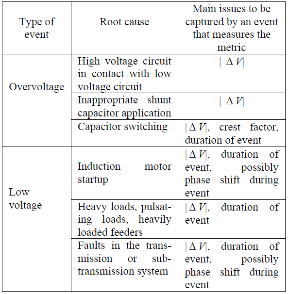
Many power quality indices relate to steady state phenomena, and relatively few relate to momentary events. However, many power quality engineers feel that bus voltage sags, a natural consequence of a highly interconnected transmission system, may be the most important type of power quality degradation, and therefore a useful measure of the severity of these events is desirable. One such metric is the power acceptability curve (or voltage sensitivity or voltage vulnerability curve) which is a graphic metric of the severity of bus voltage sags plotted versus the duration of these events. Table I shows some of the issues that might be captured by a power acceptability (sensitivity) metric.
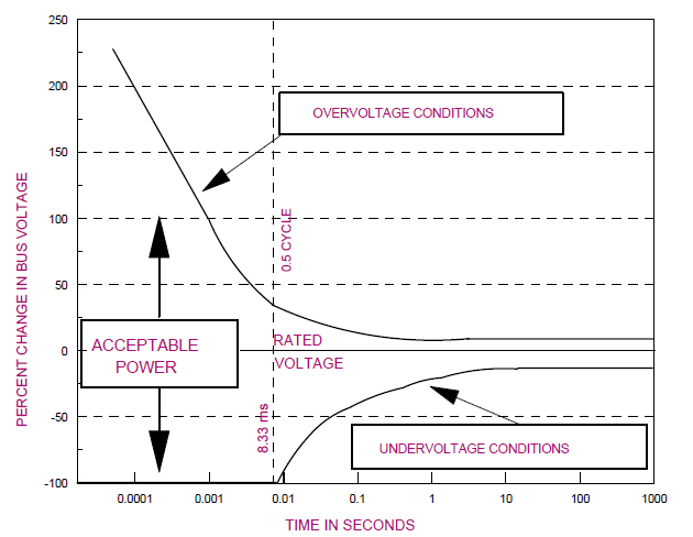
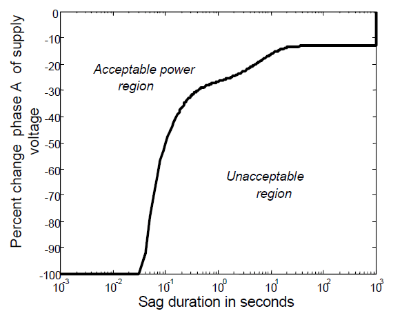
The best known of the graphical metrics for bus voltage sensitivity is the Computer Business Equipment Manufacturing Association (CBEMA) curve which is a graphic depicting the severity of a distribution bus voltage sag, Δ V, versus its duration T. The Δ V-T plane is a two dimensional space in which the line Δ V = 0 represents the case that distribution voltage is at rated value, and the Δ V < 0 half-plane is the bus voltage sag region. Overvoltage and undervoltage events of very minimal impact (small | Δ V | ) are considered ‘acceptable’ in the sense that loads are not disrupted; further, very short duration events (small T) are considered acceptable. Thus the Δ V – T plane is divided into acceptable and unacceptable regions. Fig. (1) shows the CBEMA power acceptability curve. The CBEMA curve depicted in Fig. (1) has Δ V indicated as a percent of rated voltage, and T shown on a logarithmic scale in seconds.
Table I Some issues in voltage sag and overvoltage events in primary distribution systems
Table I Some issues in voltage sag and overvoltage events in primary distribution systems
Fig. (1) The CBEMA power acceptability curve
References [1-3] discuss a fuzzy logic alternative to assess voltage – load sensitivity, testing of loads to CBEMA standards, and computer performance during voltage sags respectively. Bollen has discussed a classification system of voltage sags and their effects [4]. Ride through issues for adjustable speed drives appear in [5]. References [6] and [7] by Kyei and other researcher describe research into the ‘derivation’ of these curves by using data from appropriate models of loads.
It is evident that power acceptability curves have frailties in design and application. For example, very short duration events (e.g., less than a cycle in duration) have an ambiguity in the sense that the duration of the event may be difficult to identify, and the point on- wave of the disturbance may have significant impact on the load. Point-on-wave information is not depicted in the Δ V-T plane. Further, the three phase implications of a power acceptability curve as indicated above are not clear: should one utilize phase information in the Δ V-T plane, or the positive sequence of the distribution voltage? Or is the graph basically a single phase representation? Another commonly asked question relates to the equation of the loci shown in Fig. (1). The CBEMA curve was developed from experimental and historical data: that is, cases of load disruption of mainframe computers were plotted in the Δ V-T plane, and a separator was developed to identify the acceptable and unacceptable regions.
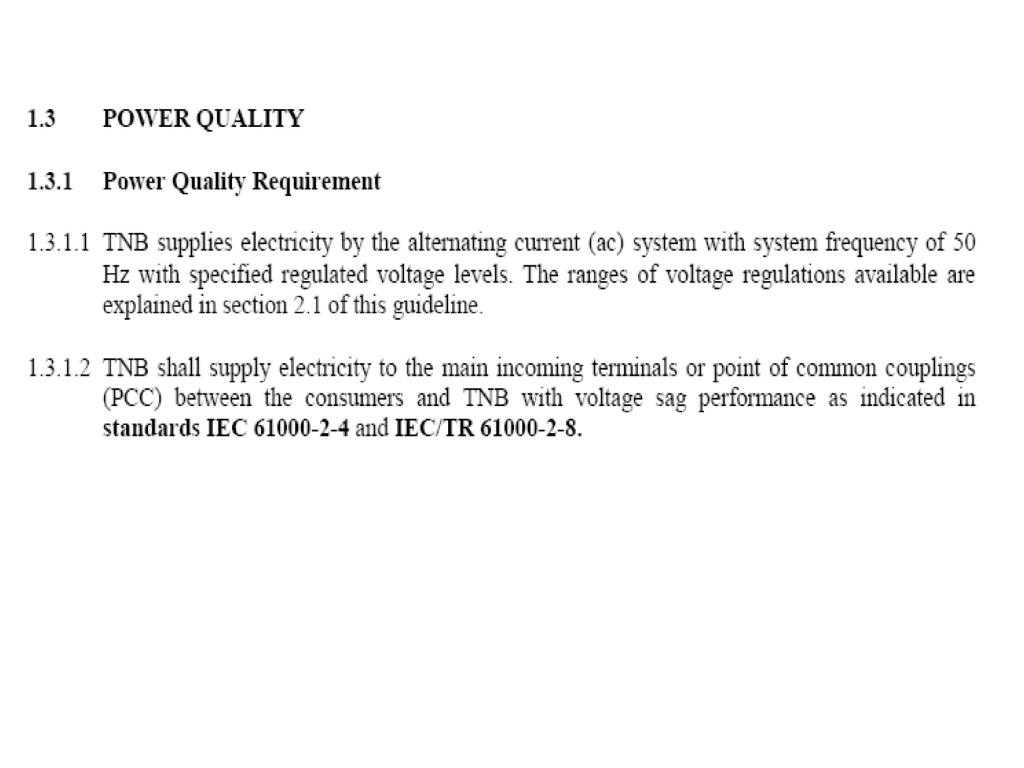
II. A power quality standard
In 1998, Ayyanar and others [7] suggested the concept of a standard to represent whether power distributed is acceptable or unacceptable. The essence of the concept is that one needs to write a concrete criterion upon which acceptability is decided. One ultimate criterion of power acceptability relates to the operating status of the industrial process.
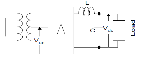
The particular power quality criterion depends on the nature of the load. For example, simple incandescent lighting loads may have a very loose criterion for acceptability, while certain sensitive computer controls may have a much more restrictive criterion. The difficulty in the selection of a single suitable criterion is confounded by the many possible load types. For simplicity, consider the rectifier load type depicted in Fig. (2). Voltage sags occur due to faults in the transmission, subtransmission, and primary distribution system, and they appear as low voltage conditions at Vac depicted in Fig. (2). If the sag is of short duration and shallow depth, the ultimate industrial process ‘rides through’ the disturbance. This means that although Vac is depressed, Vdc does not experience a sufficient disturbance to affect the load. The concept of a voltage standard is introduced at this point: a voltage standard is a criterion for power acceptability based on a minimum acceptable DC voltage at the output of a rectifier below which proper operation of the load is disrupted.
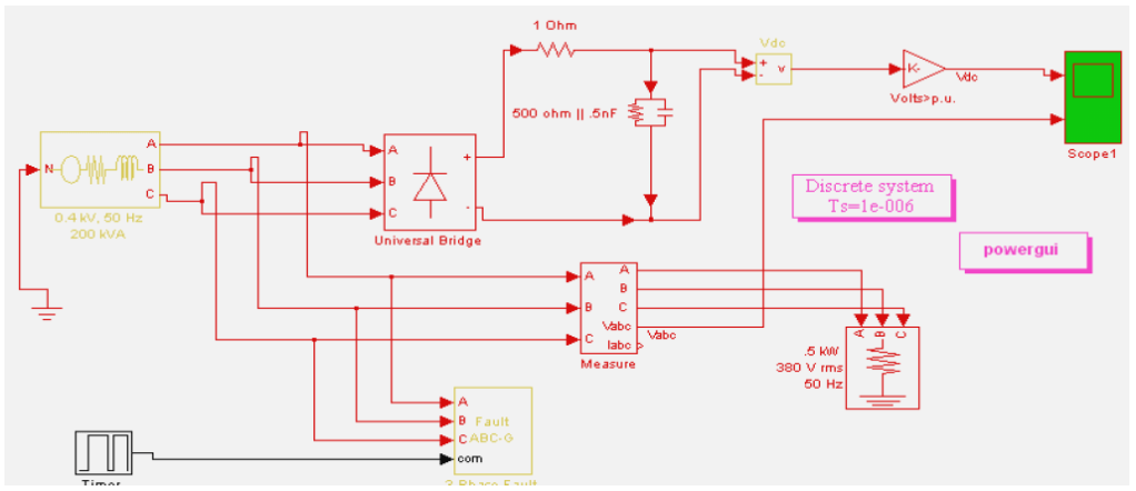
As an example of a voltage standard consider the following: if Vdc drops below 87% of rated voltage, the load is lost, and the distribution power is deemed to be unacceptable. The term ‘standard’ used in this context refers to the ultimate criterion upon which a decision of acceptability of supply is made. The use of the term ‘standard’ is not meant to imply an industry wide standard such as an IEEE standard. Fig. (3) shows a simulation study suitable for quantifying the effect of sags on rectifier load performance.
Fig. (2) A rectifier load
Fig. (3) Simulation of a three phase rectifier load
III. Analytical synthesis of the CBEMA curve
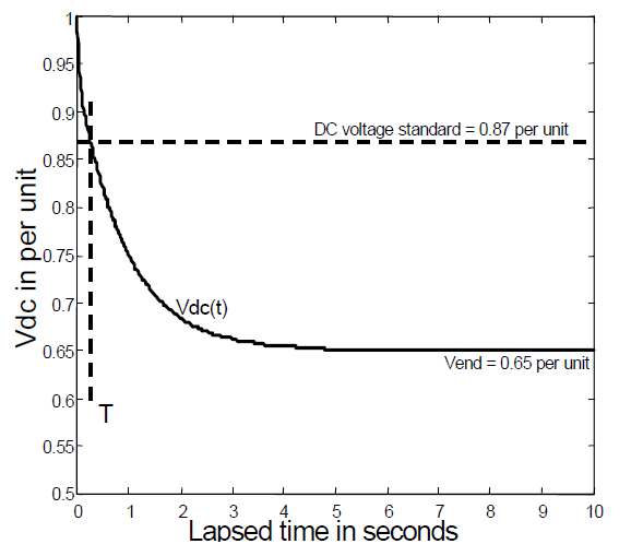
The CBEMA curve was derived from experimental and historical data taken from mainframe computers. The best engineering interpretation of the CBEMA curve can be given in terms of a voltage standard applied to the DC bus voltage of a rectifier load. Consider the case of either a single phase full wave bridge rectifier or the three phase bridge counterpart. Let the load on the DC side be an RLC load. If the DC bus voltage under a faulted condition is plotted as a function of the sag duration, the resulting curve is depicted in Fig. (4). From Fig. (4), the locus of Vdc could be represented as a double exponential in the form,
Vdc(t) = A + Be–bt + Ce-ct.
Parameter A is the ultimate (t → ∞ ) voltage, Vend, of the rectifier output. For the single phase case, and for the balanced three phase case, A is simply the depth of the AC bus voltage sag.
Fig. (4) Locus of Vdc(t) under fault conditions (at t = 0) for a single phase bridge rectifier
For more complex cases, e.g. unbalanced sags, parameter A can similarly be identified as the ultimate DC circuit voltage if the sag were to persist indefinitely (this is readily calculable by steady state analysis of the given sag condition and the rectifier type). If three points are selected on the CBEMA curve to identify the RLC filter combination used in the rectifier types considered in the original CBEMA tests, one finds,
Vdc(t) = Vend + 0.288e-1.06t + (0.712-Vend)e-23.7t. (1)
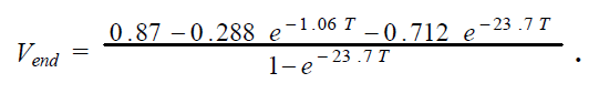
As an example, let the voltage standard be Vdc ≥ 0.87. Then the Vdc excursion becomes unacceptable at T when Vdc= 0.87 in Equation (1). Solution for Vend in terms of t = T in this expression gives
This is the formula for the undervoltage limb of the CBEMA curve (Vend in per unit, T in seconds).
IV. Some practical considerations
Application of the CBEMA curve or most other power quality ‘standards’ require certain practical considerations. Among these non-ideal considerations are:
The meaning of Δ V for short term events, especially when represented in root-mean square (RMS) values
Three phase considerations
Non ideal sags (e.g., the sag is –10% for the first few cycles, followed by –15% for the next few cycles – or even less ideal conditions in which the sag has no well defined value
Repeating events (e.g., one event, followed by restoration of normal operating conditions, followed by another event)
Point-on wave issues (see Section 5)
Multiple loads each with different sensitivity to bus voltage magnitude
Some of these issues are more easily considered than others. However, the rectifier and 87% Vdc interpretation given above do apply in all the cited practical cases. That is, at least in theory, a given non ideal, and perhaps three phase case, could be simulated utilizing a rectifier load with a DC circuit filter of the type cited above in connection with the ‘derivation of the CBEMA curve’. The three phase case is most easily considered as follows: Fig. (4) shows a power acceptability curve for a three phase rectifier. The case considered here is that of a phase A to ground fault using an 87% Vdc voltage standard. The procedure for the development of the power acceptability curve is similar to the one employed in deriving Equation (1). The unbalanced rectifier is analyzed simply, and Vdc(t) in this case is given as
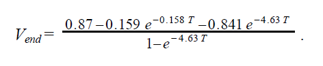
Vdc(t) = Vend + 0.159e-0.158t + (0.841-Vend)e-4.63t . (2)
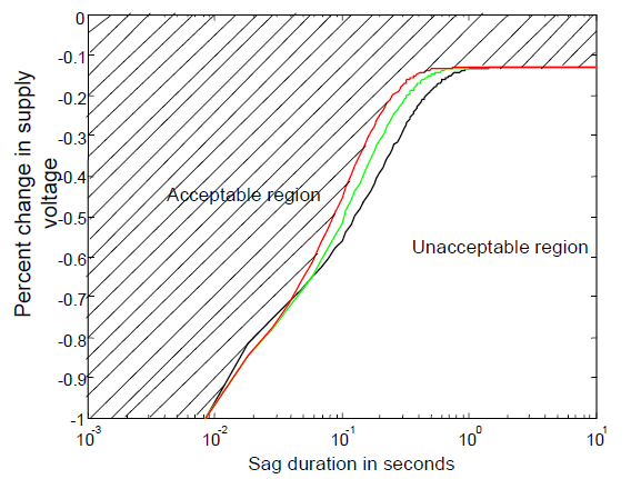
In Equation (2), the time constants were obtained using an LC filter on the DC side of a three phase, six-pulse bridge rectifier. The values of the LC were chosen to agree with the filter design used in the single phase case mentioned in connection with the derivation of Equation (1). That is, the CBEMA curve was found to correspond to the single phase rectifier case plus filter F. If filter F is used as a filter in the three phase case, Equation (2) results. Select a voltage standard of Vdc ≥ 0.87 When substituted into Equation (2) gives a formula for the power acceptability curve shown in Fig. (5) as
Other unbalanced faults are analyzed similarly.
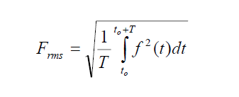
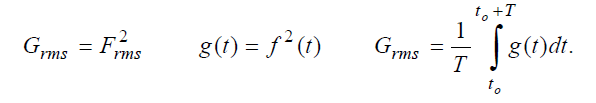
The issue of short term representation of Δ V in terms of RMS values was considered in [8]. In many power quality studies, waveforms are characterized through a RMS value,
where f(t) is a time signal and T is either the period of the time signal or a suitably long time.
Fig. (5) Power acceptability curve for a three phase rectifier load with a phase-ground fault at phase A, 87% Vdc voltage standard
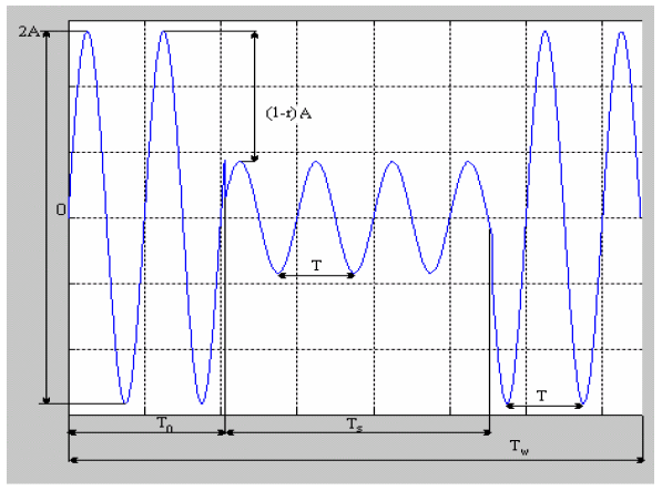
For the periodic case, when T is an integer multiple of the period of f(t), and t0 is a fixed point on the wave, the RMS value is termed a synchronous RMS (s-RMS). The s-RMS operation maps a time signal to a single point and can be visualized as an information concentrator. It is a simple matter to demonstrate that the s-RMS quantifies the Joule effect of a sinusoidal voltage or current. Reference [9] contains a discussion of applications and calculation procedures. Fig. (6) shows an example of a short term voltage sag for which the following key parameters are noted:
Tw is the length of the observation time window
Ts is the duration of the change in signal’s amplitude
T is the period of the signal, assumed as with sinusoidal variation
T0 is the moment of the amplitude change (considering that the observation window starts at t = 0)
r is the magnitude of amplitude change (in p.u.; the reference value is the amplitude at t < t0). Note that r ≤ 1 and r ≥ 0 for voltage sags, r < 0 for swells.
ϕ is the phase at t = 0.
Fig. (6) Model of a voltage sag signal
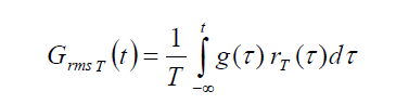
In power quality studies, the effects on consumers are often quantified in terms of the deviation of secondary distribution voltage RMS values. However when sag events are of short duration, the RMS values may have a problematic interpretation. There are many hardware and software algorithms which compute RMS values, and it becomes advisable to identify the hidden possible errors in calculation and interpretation. Note that the RMS operator is nonlinear, but working with F2rms and f2(t) gives the linear formulation,
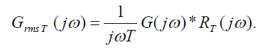
If the RMS operator is continuously carried out over a windowed time T, using past samples from the input signal g(t), a moving average finite impulse response filtering is performed,
where rT(t) is a rectangular pulse which is zero everywhere except in the interval [t–T, t] where it is unity. In the Fourier domain
The notation (*) denotes frequency domain convolution. Equation (4) indicates that there is a frequency response interpretation to the RMS operator. References [10,11] further discuss factors relating to the calculation of the RMS value.
The problem of repeated events is considered in [12]. The concept of repeated events is problematic because a second event, following closely after a first event, could have greater impact than an isolated event that is identical to the cited second event. For example, a momentary sag occurring at t = 0, for six cycles, followed by a second event at t = 0.15 s (60 Hz system) of duration six cycles might be analyzed; in such a case, the analysis of the second event of six cycles is quite different from an analysis performed of an isolated, non-repeated event of identical duration and sag depth. Heydt [12] suggests that there is a recovery time for which a system must progress in order to render an event in isolation from previous events. The concept of a recovery time is very similar to that of the ‘derivation of the CBEMA curve’ given above: that is, the recovery time of a sag can be plotted in the form of isopleths on a Δ V-T plane. The alternative, if the information is available, is to simulate the double (or triple, or multiple) event using a circuit as indicated in Figures (2) and (3).
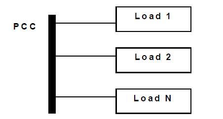
The issues of multiple loads can be depicted as Fig. (7). For such a configuration, the CBEMA curve for each load may be calculated, tailoring the curve as needed. When the resultant CBEMA curves are drawn on a common Δ V-T plane, the inner area contains the acceptable region, and the outer area is the unacceptable region as shown in Fig. (8). The area(s) between the inner and outer regions represent power acceptable to some loads, and unacceptable to others.
Fig. (7) Multiple loads at a point of common coupling (PCC)
Fig. (8) Power acceptability region for the case of multiple loads
V. Point on wave issues
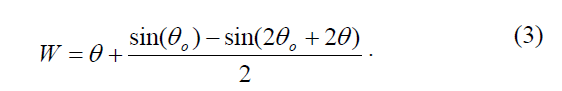
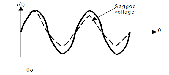
A momentary interruption of voltage or momentary sag in voltage magnitude may initiate at any point in the sinusoidal cycle as indicated in Fig. (9). For a linear load at unity power factor, the load current will be identical in phase to the indicated voltage. The energy transfer from the source to the load depends generally on θo as well as the duration of the sag. Consider a total outage of supply voltage. Integrating v(t)i(t) over θo to θo + θ where θ is the duration of the sag represented in radians assuming 60 Hz (or 50 Hz as appropriate), one finds that the energy that should have been delivered during the sag (and is now unserved due to the outage) is W,
For this simple formula, the rms supply voltage and current are both 1.0 per unit. Note that for values of θ that correspond to less than a half cycle (i.e., θ < π ), the CBEMA curve dictates that power delivery is ‘acceptable’. For longer duration outages, W depends not only on the duration of the outage θ , but also the point on wave θo at the initiation of the sag.
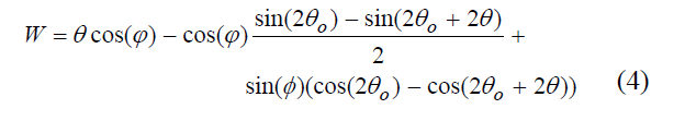
The more general case of a linear load with power factor cos(ϕ ) is more involved since the instantaneous power is a double frequency sine wave whose DC offset (i.e., the average power) is proportional to cos(ϕ ) . The unserved energy on total outage is
Collins and others have discussed the practical implications of the point on wave of the initiation of a voltage sag, including laboratory verified phenomena [13]. For long outages (largeθ , e.g., much larger than three cycles or 6π radians), the term in Equations (3) and (4) that is proportional to θ dominates, and the unserved energy is no longer greatly dependent on the point on wave at the sag initiation.
Fig. (9) Point on wave initiation of a voltage sag event
VI. A single index to show compliance with CBEMA
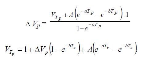
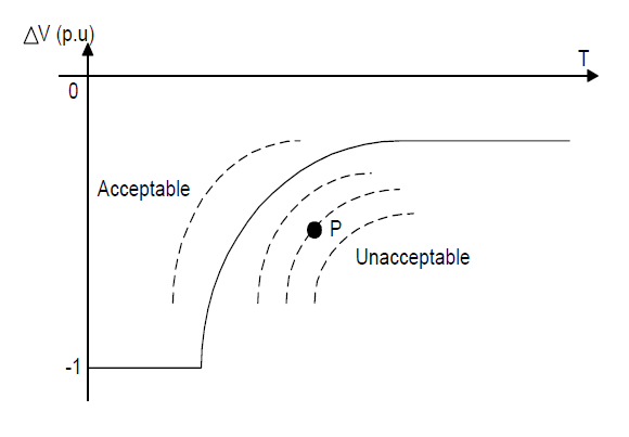
In most areas of engineering, it is important to use indices to measure or quantify the quality of performance. Power acceptability curves graphically depict power quality; but is there an index that can be used to assess “acceptability” or “unacceptability”? Consider Fig. (10) in this matter. Point P represents an event Δ V = Δ Vp and T = Tp (shown as ‘unacceptable’ in Fig. (10)). As an index of power acceptability, it is proposed to vary the threshold VT until the power acceptability curve passes through P. This is shown as dashed lines in Fig. (10). Then, one sets VT to VTp ,
Fig. (10) Graphic interpretation of an index of power acceptability for an event P
Consider the index VTp / VT . If VTp / VT ≥ 1, the point P represents an acceptable event. It is a simple matter to show that the theoretical maximum of the index VTp / VT is 1/VT . Introduce the notation Ipa for the new index,
Ipa = VTp / VT.
If one uses the notation Tx as the maximum time for which acceptable power is attained upon a total outage (i.e., Δ V = -1),
This is an index of power acceptability for the event P. When the index is greater than unity, one is in the acceptable power region, and when the index is below unity, one is in the unacceptable region. At unity itself, the event is exactly on the CBEMA curve.
VII. Recommendations and concluding comments
In this paper, the CBEMA curve was revisited and the curve was analytically synthesized using a new concept, the voltage standard. The standard refers to an ultimate criterion that power is unacceptable if the DC voltage of a certain rectifier load drops below 87% of rated value. A double exponential equation describing the CBEMA curve is developed. This provides a useful method to consider the effect of unbalanced voltage sags and to develop CBEMA-like curves for other types of loads. A scalar index of compliance termed Ipa has been illustrated. This index is based on the CBEMA curve compliance.
Additional practical considerations relating to power acceptability include:
The meaning of Δ V for short term events, especially when represented in root-mean square (RMS) values
Three phase considerations
Non ideal sags
Repeating events
The energy served to a load during a sag as a function of the point-on-wave of the initiation of the event
Multiple loads each with different sensitivity to bus voltage magnitude.
It appears that the main advantage of the CBEMA curve is the ease in application, and also in the familiarity of the concept by most power engineers.
Although accuracy of the curve in predicting true acceptability – unacceptability of the power supply may not be a strong point of CBEMA technology, at least some problematic issues of its application may be resolved using the concept of a voltage standard.
Acknowledgements
The authors gratefully acknowledge the support of the Power Systems Engineering Research Center (PSerc) and SRP. Most of the work represented here came from Mr. John Kyei of the California ISO, Folsom CA. Dr. Raja Ayyanar of Arizona State University originated the concept of the voltage standard, and the authors acknowledge his contribution. Dr. Albu acknowledges the support of the Fullbright Fellowship.
References
[1] B. Bonatto, T. Niimura, H. Dommel, “A fuzzy logic application to represent load sensitivity to voltage sags,” Proceedings International Conference on Harmonics and Quality of Power, October, 1998, pp. 60-64. [2] E. Collins, R. Morgan, “A three phase sag generator for testing industrial equipment,” IEEE Transactions on Power Delivery, v. 11, No. 1, January, 1996, pp. 526 – 532. [3] D. Koval, “Computer performance degradation due to their susceptibility to power supply disturbances,” Conference Record, IEEE Industry Applications Society Annual Meeting, October, 1989, v. 2, pp. 1754 – 1760. [4] M. Bollen, L. Zhang, “Analysis of voltage tolerance of AC adjustable-speed drives for three-phase balanced and unbalanced sags,” IEEE Transactions on Industry Applications, v. 36, No. 3, May-June 2000, pp. 904 – 910. [5] E. Collins, A. Mansoor, “Effects of voltage sags on AC motor drives,” Proceedings of the IEEE Technical Conference on the Textile, Fiber and Film Industry, 1997, pp. 9 – 16. [6] J. Kyei, “Analysis and design of power acceptability curves for industrial loads,” MSEE Thesis, Arizona State University, Tempe AZ, December 2001. [7] J. Kyei, R. Ayyanar, G. Heydt, R. Thallam, J. Blevins, “The design of power acceptability curves,” accepted for publication, IEEE Trans. on Power Delivery, 2003. [8] M. Albu, G. Heydt, “On the use of RMS values in power quality assessment,” accepted for publication, IEEE Trans. on Power Delivery, 2003. [9] S. Kuo, B. Lee, Real-Time Digital Signal Processing. Implementations, Applications, and Experiments with the TMS320C55X, John Wiley and Sons, New York, 2001. [10] S. Herraiz-Jaramillo, G. Heydt, E. O’Neill-Carrillo, “Power quality indices for aperiodic voltages and currents,” IEEE Transactions on Power Delivery, v. 15, No. 2, April 2000, pp. 784 790. [11] N. Tunaboylu, E. Collins, P. Chaney, “Voltage disturbance evaluation using the missing voltage technique,” Proceedings of the 8th International Conference on Harmonics and Quality of Power 1998, pp. 577 – 582. [12] G. T. Heydt, Computer Analysis Methods for Power Systems, Second edition, Stars in a Circle Publications, Scottsdale, AZ, 1996. [13] E. R. Collins, M. A. Bridgwood, “The impact of power system disturbances on AC-coil contactors,” Proceedings of the IEEE Technical Conference on the Textile, Fiber and Film Industry, 1997, pp. 2-6.
Published by Mirus International Inc., [2010-01-08] MIRUS-FAQ001-B2, FAQ’s Harmonic Mitigating Transformers, 31 Sun Pac Blvd., Brampton, Ontario, Canada. L6S 5P6.
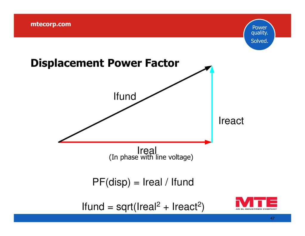
Power factor is a measure of how effectively a specific load consumes electricity to produce work. The higher the power factor, the more work produced for a given voltage and current. Figure 3-1 shows the power vector relationships for both linear and non-linear loads. Power factor is always measured as the ratio between real power in kilowatts (kW) and apparent power in kilovoltamperes (kVA).
Figure 3- 1: Power factor relationship for Linear and Non-linear loads
For linear loads, the apparent power in kVA (S = V•I) is the vector sum of the reactive power in kVAR (Q) and the real power in kW (P). The power factor is P/S = CosΦ, where Φ is the angle between S and P. This angle is the same as the displacement angle between the voltage and the current for linear loads. For a given amount of current, increasing the displacement angle will increase Q, decrease P, and lower the PF. Inductive loads such as induction motors cause their current to lag the voltage, capacitors cause their current to lead the voltage, and purely resistive loads draw their current in-phase with the voltage. For circuits with strictly linear loads (a rare situation) simple capacitor banks may be added to the system to improve a lagging power factor due to induction motors or other lagging loads.
For non-linear loads, the harmonic currents they draw produce no useful work and therefore are reactive in nature. The power vector relationship becomes 3 dimensional with distortion reactive power, H, combining with both Q and P to produce the apparent power which the power system must deliver. Power factor remains the ratio of kW to kVA but the kVA now has a harmonic component as well. True power factor becomes the combination of displacement power factor and distortion power factor. For most typical non-linear loads, the displacement power factor will be near unity. True power factor however, is normally very low because of the distortion component. For example, the displacement power factor of a personal computer will be near unity but its total power factor is often in the 0.65 – 0.7 range. The best way to improve a poor power factor caused by non-linear loads is to remove the harmonic currents.
Most Utilities charge their customers for energy supplied in kilowatt-hours during the billing period plus a demand charge for that period. The demand charge is based upon the peak load during the period. The demand charge is applied by the utility because it must provide equipment large enough for the peak kVA demand even though the customer’s power demand may be much lower. If the power factor during the peak period (usually a 10 minute sliding window) is lower than required by the utility (usually 0.9 or 0.95), the utility may also apply a low PF penalty charge as part of the demand charge portion of the bill.
Suppose the peak demand was 800kW with apparent power consumption of 1000kVA (a PF of 0.8). If a power factor penalty was applied at 0.9, the Utility would charge the customer as if his demand was 0.9 x 1000kVA = 900kW even though his peak was really 800kW, a penalty of 100kW. Improving the power factor to 0.85 at 1000kVA demand would lower the penalty to just 50kW. For power factors of 0.9 to 1.0, there would be no penalty and the demand charge would be based upon the actual peak kW. The demand charge is often a substantial part of the customer’s overall power bill, so it is worthwhile to maintain good power factor during peak loading and reducing the harmonic current as drawn by the loads can help achieve this.
References:
1. Roger C. Dugan, Electrical Power Systems Quality, McGraw-Hill, New York NY, 1996, pp. 130-133 2.H. Rissik, The Fundamental Theory of Arc Convertors, Chapman and Hall, London, 1939, pp 85-97
Harmonics and Harmonic Mitigating Transformers (HMT’s) Questions and Answers
This document has been written to provide answers to the more frequently asked questions we have received regarding harmonics and the Harmonic Mitigating Transformer technology used to address them. This information will be of interest to both those experienced in harmonic mitigation techniques and those new to the problem of harmonics. For additional information visit our Website at www.mirusinternational.com.
Published by 1Vima P. Mali, 2R. L. Chakrasali, 1K. S. Aprameya, 1Electrical and Electronics Engineering Research Centre, University B.D.T. College of Engineering, Davanagere, India. 2Department of Electrical and Electronics Engineering, SDM College of Engineering and Technology, Dharwad, India.
Research PaperSource: American Journal of Engineering Research (AJER) 2015. American Journal of Engineering Research (AJER) e-ISSN: 2320-0847 p-ISSN : 2320-0936 Volume-4, Issue-10, pp-60-68 www.ajer.org
Abstract: Voltage sag is regarded as one of the most harmful power quality disturbances due to its costly impact on sensitive loads. The vast majority of the problems occurring across the utility, transmission and industrial sides are voltage sags. The source of sag can be difficult to locate, since it occurs either inside or outside facilities. So, this paper analyses some aspects of voltage sag such as the cost of voltage sag, their characteristics, types of voltage sag, its occurrence, percentage of sag present in power system, acceptable level of voltage sag curve, voltage sag indices, its economical impact, ways to mitigate the voltage sag and finally few devices used to mitigate voltage sag.
Keywords: Voltage sag, impact, types, occurrence etc.
I. INTRODUCTION
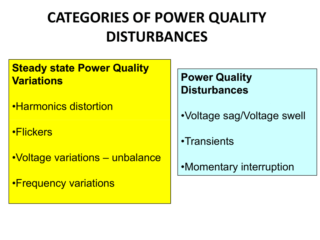
The name power quality has become one of the most productive concepts in the power industry since late 1980s. Power quality is the “Degree to which both the utilization and delivery of electric power affects the performance of electrical equipment” [1].Power quality is decided by magnitude of voltage and frequency. Voltage quality problem is divided into under voltage, overvoltage, interruption, voltage sag, voltage swell and so on, and frequency quality problem could be classified into frequency variations, transient, harmonics, etc. [2].
Voltage sag or Voltage dip the two terms are equivalent. According to the IEEE defined standard (IEEE Std. 1159, 1995), voltage sag is the decrease of rms value of voltage from 0.1 to 0.9 per unit (pu), for a duration of 0.5 cycle to 1 minute. The International Electrotechnical Commission, IEC, has the following definition for a dip (IEC 61000-2-1, 1990). “A voltage dip is a sudden reduction of the voltage at a point in the electrical system, followed by a voltage recovery after a short period of time, from half a cycle to a few seconds”. Voltage sags are present in power systems, but only during the past decades customers are becoming more sensitive to the inconvenience caused [3].
Voltage sag can cause serious problems to sensitive loads, because these loads often drop off-line due to voltage sag. As a result, some industrial facilities experience production outage that results in economic losses [4, 5, 6]. In several processes such as semiconductor manufacturing or food processing plants, the voltage dip of very short duration can cost a substantial amount of money [7]. Voltage dip is the main power quality problem for the semiconductor and continuous manufacturing industries, and also to the hotels and telecom sectors [8].
International Joint Working Group (JWG) C4.1110 sponsored by CIGRE, CIRED and UIE has addressed a number of aspects of the immunity of equipment and installations against voltage dips and also identified areas were additional work is required. The work took place between 2006 and 2009 and resulted in a technical brochure distributed via CIGRE and UIE [9]. Voltage sag on a power grid can affect facilities within a 100-mile radius. According to Electric Power Research Institute the voltage sag causes 92% of distribution & transmission power quality problems.
A typical electric customer in the U.S experiences 40 to 60 sag events per year with those events resulting in the voltage dropping to between 60 to 90% and lasting several cycles to more than a second. The large majority of faults on a utility system are single line-to-ground faults (SLGF). Three phase faults can be more severe, but much less common. System wide, an urban customer on average may see 1 or 2 interruptions a year whereas the same customer may experience over 20 voltage sag occurrences a year depending on how many circuits are fed from the substation.
II. COST OF VOLTAGE SAG
Voltage sag lasting for a few cycles result in losses of several million dollars includes:
a. Repairs cost. b. Increased buffer inventories. c. Product quality issues affect brand name, fame of the industry and even the country. d. Customer dissatisfaction due to huge loss in business. e. Penalties and disposal fees. f. Product-related losses, such as loss of product/materials, hampered production capacity, disposal charges, and increased inventory requirements. g. Labor-related losses, such as idle employees, overtime, cleanup and repair. h. Ancillary costs, such as damaged equipment, lost opportunity cost and penalties due to shipping delays.
III. CHARACTERISTICS OF VOLTAGE SAG
The magnitude of voltage and the frequency are the parameters that specify the voltage sag.
a. Magnitude:
Figure 1. Voltage sag characteristics
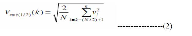
The sag magnitude is the minimum of rms voltage and refers to the retained voltage or to the drop of the voltage (IEEE P1564). Thus, a 70% sag in a 230-V system indicates the voltage dropped to 161 V. One could be tricked into thinking that 70% sag refers to a drop of 70%, thus a remaining voltage of 30% [10].The most common approach to obtain the sag magnitude is to use rms voltage. There are other alternatives, e.g. rms voltage of fundamental component and peak voltage [11,12].The rms voltage is calculated over one cycle using equation 1
The rms value using one half cycle is given by equation 2
Where N is the number of samples per cycles, V(i) is the instantaneous sampled voltage and k is the instant when the rms voltage is estimated.
b. Duration: Sag duration is commonly determined by the speed of the fault clearing time. The voltage sag duration is nothing but the period of time in which the voltage is lower than the stated limit; normally sag duration is less than 1 second (IEEE Std. 493, 1997). According to IEEE Std. 1159, 1995 voltage sag has been classified into three types based on their duration i) Instantaneous (0.5-30cycle) ii) Momentary (30 cycles-3sec) iii) Temporary (3sec-1min). For measurements in the three-phases systems the three rms voltages have to be considered to determine duration of the sag. The voltage sag starts when at least one of the rms voltages drops below the sag-starting threshold. The sag ends when all three voltages have recovered above the sag-ending threshold.
c. Unbalance of Sag: In the power system the faults are classified as symmetrical (balanced) and unsymmetrical (unbalanced) depending on the type of fault. If three phase fault occurs, the sag will be symmetrical but if the fault is single phase, double phase or double phase to ground faults the sag in three phases will not be symmetrical.
d. Phase-Angle Jump: A short circuit in a power system not only causes voltage sag, but also changes the phase angle of the voltage leading to phase-angle jump. The phase-angle jump is visible in a time-domain plot of the sag as a shift in voltage zero-crossing between the pre-event and the during-event voltage. If source and feeder impedance have equal X/R ratio, there will be no phase-angle jump in the voltage at the Point of Common Coupling. This is the case for faults in transmission systems, but normally not for faults in distribution systems. The distribution systems may have phase-angle jumps up to a few tens of degrees.
For unsymmetrical faults, the analysis becomes much more complicated. A consequence of unsymmetrical faults (single-phase, phase-to-phase, two-phase-to-ground) is that single-phase load experiences a phase-angle jump even for equal X = R ratio of feeder and source impedance. From the measured voltage wave shape, the phase angle of the voltage during the event must be compared with the phase angle of the voltage before the event.
IV. TYPES OF VOLTAGE SAG
Based on the phases affected during the sag, the voltage sag has been classified into three types:
a. Single Phase Sags: The frequently occurring voltage sags are single phase events which are basically due to a phase to ground fault occurring somewhere on the system. On other feeders from the same substation this phase to ground fault appears as single phase voltage sag. Typical causes are lightning strikes, tree branches, animal contact etc. It is common to see single phase voltage sags to 30% of nominal voltage or less in industrial plants.
b. Phase to Phase Sags: The two phase or phase to phase sags are caused by tree branches, adverse weather, animals or vehicle collision with utility poles. These types of sags typically appear on other feeders from the same substation.
c. Three Phase Sags: These sags are caused by switching or tripping of a 3 phase circuit breaker, switch or recloser which will create three phase voltage sag on other lines fed from the same substation. Symmetrical 3 phase sags arise from starting large motors and they account for less than 20% of all sag events and are usually confined to an industrial plant or its immediate neighbors.
V. OCCURRENCE OF VOLTAGE SAG
Voltage sag occurs at almost all locations in the power system and avoiding them is only practically possible up to a certain extent. Voltage sag is caused by faults on the system, transformer energizing, or heavy load switching. Reducing the number and severity of voltage sag experienced by a customer, beyond what is normally considered as good engineering practice, can be very expensive [11].
Utility side voltage sag occurs due to operation of reclosers & circuit breakers, equipment fails( due to overloading, cable faults), bad weather (thunderstorms and lightning strikes cause a significant number of voltage sags), animals & birds(squirrels, raccoons and snakes occasionally find their way onto power lines or transformers and can cause a short circuit or either phase to phase or phase to ground), Vehicles occasionally collide with utility poles (causing lines to touch, protective devices trip and voltage sags occur), Construction activity( Digging foundations for new building construction can result in damage to underground power lines and create voltage sags).
Salt spray builds up on power line insulators over time in coastal areas, even many miles inland, can cause flash over especially in stormy weather. Dust in arid inland areas can cause similar problems. As circuit protector devices operate voltage sags appear on other feeders. If electrical equipment fails due to overloading, cable faults etc., protective equipment will operate at the sub-station and voltage sags will be seen on other feeder lines across the utility system.
Industrial side voltage sags occurs within an industrial facility (due to factory equipment, office equipment, air conditioning & elevator drive motors) or a group of facilities by the starting of large electric motors either individually or in groups. The large current inrush on starting can cause voltage sags in the local or adjacent areas even if the utility line voltage remains at a constant nominal value. Starting a large load, such as an electric motor or resistive heater, typically draw 150% to 500% of their operating current as they come up to speed. Resistive heaters typically draw 150% of their rated current until they warm up. Even 80% of all power quality problems occur in a company’s distribution and grounding/bonding systems.
Electronic process controls, sensors, computer controls, PLC’s and variable speed drives, conventional electrical relays are all to some degree susceptible to voltage sags. In many cases one or more of these devices may trip if there is a voltage sag to less than 90% of nominal voltage even if the duration is only for one or two cycles i.e. less than 100 milliseconds. The time to restart production after such an unplanned stoppage can typically be measured in minutes, hours or even days. Costs per event can be many tens of thousands of dollars. Voltage sag cannot be eliminated fully so, Industrial customers who have invested heavily in production equipment which is susceptible to voltage sags must take responsibility for their own solutions to voltage sags or lose some benefit from their investment.
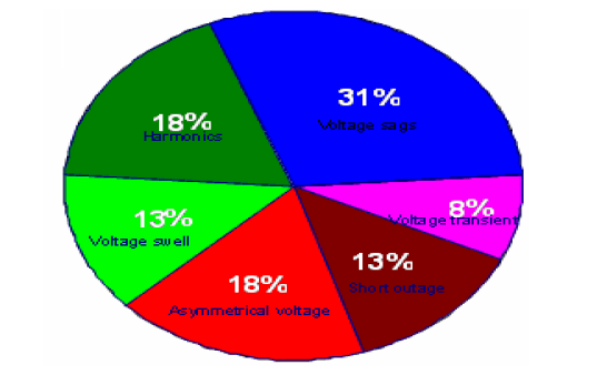
VI. PERCENTAGE OF SAG PRESENT IN POWER SYSTEM
The most common types of voltage abnormalities are: harmonics, voltage sags, voltage swells and short interruptions. Among these, voltage sags account for the highest percentage of occurrences in equipment interruptions, as shown in Figure 1. The figure 1 indicates that voltage sags account for the highest percentage of equipment interruptions, i.e., 31%. Voltage sags are also major power quality problem that contributes to nuisance tripping and malfunction of sensitive equipment in industrial processes and Table 1 below gives causes of voltage sag on distribution system based on number of voltage sag occurrences and its percentage.
Figure 1 Power quality disturbances [28]
Table 1. Causes of voltage sag on distribution system
VII. CLASSIFICATION OF VOLTAGE SAG
There are two methods for classification the three phase voltage sags i) ABC Classification (First method) ii) Symmetrical Components (Second method). Due to simplicity, first method is more used than the symmetrical components classification. However, this classification is based on a simplified model of the network and it is not recommended to use for the classification of voltage sags obtained from measured instantaneous voltages.
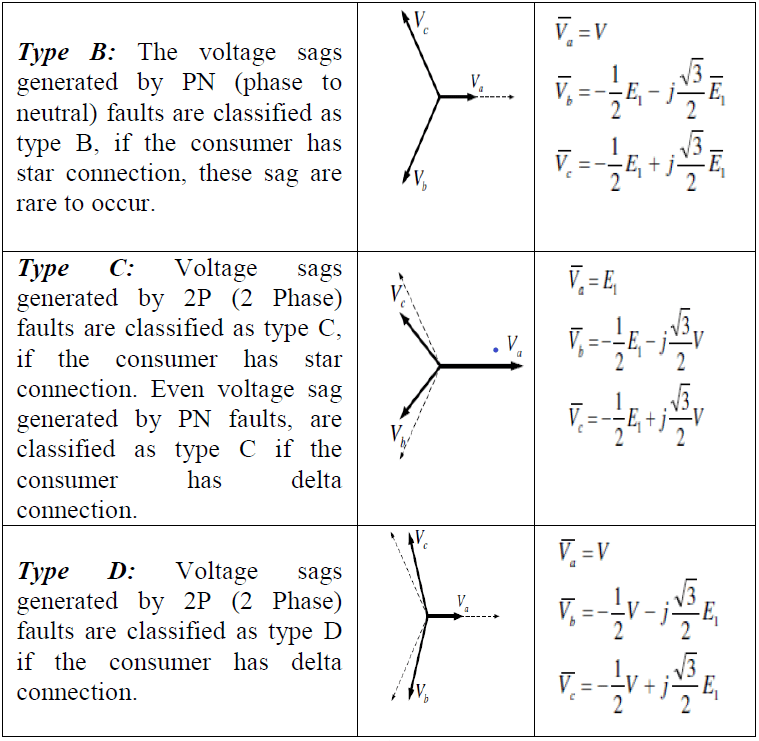
In the first classification, in 1997, Bollen has proposed a four type’s classification for voltage sags (A, B, C, D) based on type of fault which generates the sag [13]. This classification isn’t so good for voltage sags generated by 2PN (2 phase to neutral) faults [14, 15]. So, Bollen has proposed a new by adding another three (E, F, G) types of voltage sags. Types of voltage sag are:
Table 2. The phasor diagram and equations
The pre-event voltage in phase A is denoted as E1, recalling to the equivalence between phase A voltage and positive sequence voltage in a balanced system. The voltage in the phase that has experienced the sag or between the phases that has experienced the sag is indicated as V. In table 1 sag types are shown considering phase A as the reference phase. It means that another set can be derived for phase B or C are set as the reference phase. This classification is the base for international standard IEC 61000-4-11[18], because it makes possible generation of the seven types of voltage sag.
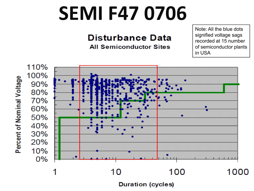
VIII. ACCEPTABLE LEVEL OF VOLTAGE SAG CURVE
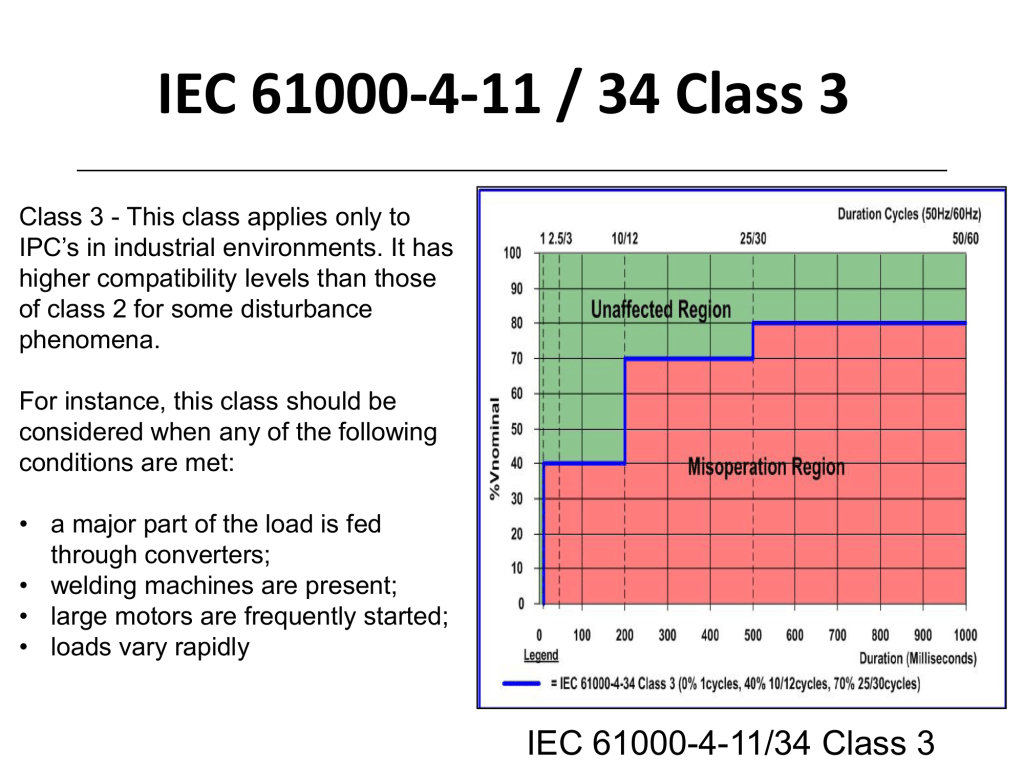
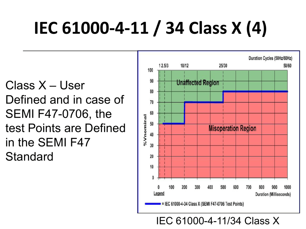
This is generally determined by power quality curves, a plot of voltage magnitude versus time. Power quality curves represent the intensity and duration of voltage disturbances. The Computer and Business Equipment Manufacturers’ Association (CBEMA), and Semiconductor Equipment and Materials Institute (SEMI) have published information defining what levels of poor power quality, specifically voltage sag, equipment should be able to tolerate. Other power quality curves in common use today were developed by the American National Standards Institute (ANSI) and the Information Technology Industry Council (ITIC).
The ANSI curves plot the deviation from nominal voltage as a percentage of nominal voltage compared to the duration or the maximum length of time the voltage is permitted to reach. For example, the limit for voltage occurrences greater than 1 second duration might be ± 10%. The ITIC and CBEMA curves also plot voltage with respect to duration, but as a percentage of absolute voltage. Electronic equipment can typically withstand high voltages provided they last for less than 1 millisecond in duration, but voltages greater than +10% or -20% for between 0.5 seconds and 10 seconds duration are to likely create problems.
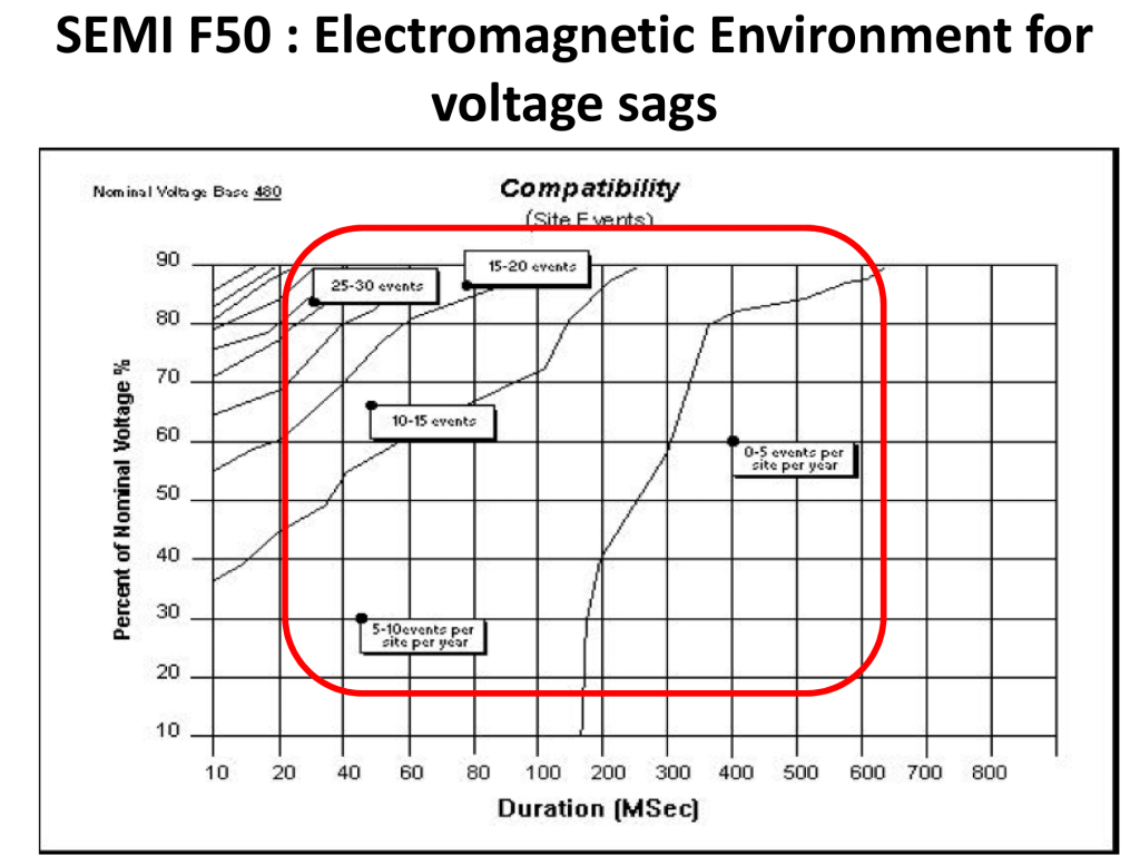
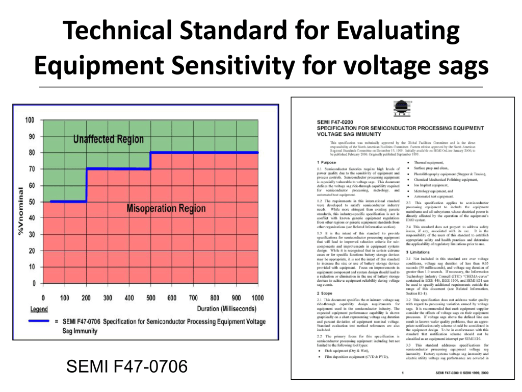
ITIC also shows that computer equipment should be able to ride through short-duration voltage sags, if the voltage doesn’t go below 70%. For sags of longer duration, voltages below 80% could affect the equipment. Even SEMI F47 semiconductor industry standard specifies an improved voltage sag ride-through for process tools. It requires a ride-through down to 50% voltage for 200 milliseconds, which will significantly reduce the number of voltage sags that may cause process disruptions in semiconductor plants. These curves are merely guidelines, and some electronic equipment may require higher power quality conditions than those represented in these standards.
IX. VOLTAGE SAG INDICES
PQ indices are key issue to indicate the different performance experienced at the transmission, sub-transmission, substation and distribution circuit levels. There are various ways of presenting voltage sag performance [16].
a.SARFI (System Average Rms Variation Frequency Index)
b.SIARFI (System Instantaneous Average Rms Variation Frequency Index)
c.SMARFI (System Momentary Average Rms Variation Frequency Index)
The most common index use is the SARFI. This index represents the average number of voltage sags experienced by a end user each year with a specified characteristic. For SARFI_X, the index would include all of the voltage dips where the minimum voltage was less than X(where X is a number between 0 and 100) gives the number of events with a duration between 10 milliseconds and 60 seconds and a retained voltage less than X%. SARFI_70 gives the number of events with retained voltage less than 70% [17, 18]. Standard voltage thresholds are 140, 120, 110, 90, 80, 70, 50, and 10 % of nominal.
X. ECONOMICAL IMPACT OF VOLTAGE SAG
The cost associated with the voltage sag is more compared to other power quality issues:
a. The cost to North American industry of production stoppages caused by voltage sags now exceeds U$250 billion per annum [9].
b. In South Africa, a recent study showed that major industries suffer annual losses of more than 200 US$ million due to voltage sag problems [11].
c. A study in United States (U.S.), the total damage by voltage sag may amount to 400 Billion Dollars [12].
d. Manufacturing facilities have cost ranging up to millions of dollars attributed to a single disruption of the process whereas the cost to commercial customer (e.g., banks, data center, customer service centers, etc.) can be just as high if not higher [14].
e. In automotive industry, four-cycle voltage sag can lost over 700,000 US$ in the following 72 minutes due to shut down of process and required rework from malfunction of programmable controllers and drive systems working in a real-time process environment [19].
f. One automaker estimated that the total losses from momentary voltage sag at all its plants runs to about $10M a year [1].
g. Manufacturing facilities have costs ranging from Rs.4, 00,000 to millions of rupees associated with a single interruption to the process. Momentary interruptions or voltages sags lasting less than 100 ms can have the same impact as in outage lasting many minutes [20].
h. If an interruption costs Rs.16, 00,000, the total costs associated with voltage sags and interruptions would be Rs.2, 70, 40,000/-year. (The total cost is appro. 17 times the cost of an interruption) [21].
The table 3 shows some industries and their loss per event due to voltage sag and table 4 shows Cost of Momentary interruption due to voltage sag.
Table 3. Industries and their loss per event
Sl.No
Industry
Loss per event (US$)
1.
Semiconductor industry
2,500,000
2.
Credit card processing
250,000
3.
Equipment manufacturing
100,000
4.
Automobile industry
75,000
5.
Chemical industry
50,000
6.
Paper Manufacturing
30,000
Table 4. Shows industries & their Cost of Momentary interruption [22]
Cost of Momentary interruption
Cost of Momentary interruption
Sl.No
Industry
Minimum
Maximum
1.
Semiconductor Manufacturing
$20.0
$60.0
2.
Pharmaceutical
$5.0
$50.0
3.
Electronics
$8.0
$12.0
4.
Communications, Information Processing
$1.0
$10.0
5.
Automobile manufacturing
$5.0
$7.5
6.
Food processing
$3.0
$5.0
7.
Glass
$4.0
$6.0
8.
Petrochemical
$3.0
$5.0
9.
Textile
$2.0
$4.0
10.
Rubber & plastics
$3.0
$4.5
11.
Metal fabrication
$2.0
$4.0
12.
Mining
$2.0
$4.0
13.
Hospitals, Banks, Civil services
$2.0
$3.0
14.
Paper
$1.5
$2.5
15.
Printing (News Paper)
$1.0
$2.0
16.
Restaurants, bars, hotels
$0.5
$1.0
17.
Commercial shops
$0.1
$0.5
XI. MITIGATION OF VOLTAGE SAG
There are several ways to mitigate the voltage sag:
a. From Fault to Trip: The equipment trip is the main cause of voltage sag, if there are no equipment trips due to short-circuit fault, there is no voltage sag problem. Due to short circuit at the fault position, the voltage drops to zero, or to a very low value. This zero voltage is changed into an event of a certain magnitude and duration at the interface between the equipment and the power system. If the fault takes place in a radial part of the system, the protection intervention clearing the fault will also lead to an interruption. If there is sufficient redundancy present, the short circuit will only lead to voltage sag. If the resulting event exceeds a certain severity, it will cause an equipment trip. The equipment trip due to short circuit fault can be minimized by:
Reducing the fault-clearing time.
Changing the system such that short-circuits faults result in less severe events at the equipment terminals or at the customer interface.
Connecting mitigation equipment between the sensitive equipment and the supply.
Improving the immunity of the equipment.
b. Reducing the Number of Faults: Short circuits cannot be entirely eliminated. The majority of failures are due to faults on one or two distribution lines. Below mentioned fault mitigation measures may be expensive, especially for transmission systems but their costs have to be weighed against the consequences of the equipment trips. The actions taken are:
Replacing overhead lines with cables.
The use of insulated conductors on overhead lines.
Regular tree cutting in the area of the transmission line and fencing against animal.
Shielding overhead conductors with additional shield wires and by increasing insulation level.
Increased frequency of overhaul and periodic maintenance, cleaning insulators etc.
c. Reducing the Fault-Clearing Time: To minimize the fault clearing time several types of fault current limiters(able to clear a fault within one half-cycle) are in use for low and medium voltages system i.e. few tens to kilovolts, but actually they do not clear the fault, they only reduce the current magnitude within one or two cycles. Reducing the fault clearing time of any event does not reduce the number of events occurring, but can reduce the severity of fault impact. Recently introduced static circuit breaker has the same characteristics as fault current limiters. Fault-clearing time is not only the time needed to open the breaker, but also the time needed for the protection to make a decision.
d. Changing the Power System: The cost associated with changing the supply system may be high, especially for transmission and sub transmission voltage levels. But in case of industrial systems, the design stage will outweigh the cost. Some other ways to mitigate the voltage sags are:
By installing a generator near the sensitive load. The generators will keep up the voltage during remote sag.
Split buses or substations in the supply path to limit the number of feeders in the exposed area.
Determine the frequency, depth & duration of the voltage sag. Collection of data is essential if the optimal solution is to be determined.
In order to provide a cost effective solution to voltage sag problems, it is necessary to determine which equipment is more subjected to voltage sag.
XII. INSTALLING VOLTAGE SAG MITIGATING EQUIPMENT
There are number of mitigating devices used to mitigate the voltage sag:
a. Device Voltage Restorer (DVR): DVR uses modern power electronic components to insert a series voltage source between the supply and the load. The voltage source compensates for the voltage drop due to the sag. The DVR is a series connected facts device to protect sensitive loads from supply side disturbances; it can also act as a series active filter, isolating the source from harmonics generated by loads. This is often the best solution when voltage sags are the dominant concern. DVR is also used for protecting individual loads or group of loads.
b. Uniform Power Quality Conditioner (UPQC): is the integration of series and shunt active filters, connected back to back on the dc side and share a common DC capacitor. The series connected UPQC is responsible for mitigation supply side disturbances such as voltage sags, flickers, voltage unbalance and harmonics. The shunt component is responsible for mitigating the current quality problems caused by consumer: poor power factor, load harmonic currents, load unbalance etc. It can perform the function of both DSTATCOM and DVR [23].
c. Uninterruptable Power Supply (UPS): Utilize batteries to store energy that is converted to a usable form during outage or voltage sag. This is the most commonly used device to protect low-power equipment (computers, etc.) against voltage sags and interruptions. During the sag or interruption, the power supply is taken over by an internal battery. The battery can supply the load for, typically, between 15 and 30 minutes.
d. Motor-Generator Sets (M-G Sets): It usually utilizes flywheels for energy storage. They completely decouple the load from the electric power system. Rotational energy in the flywheel provides voltage regulation and voltage support during under voltage conditions. M-G sets have relatively high efficiency and low initial capital cost. They are only suitable for industrial environment due to noise and the maintenance required compare to office environment.
e. Ferro resonant, Constant Voltage Transformers (CVTs): can be used to improve voltage sag ride through capability. CVTs are especially attractive for constant, low power loads, variable loads, especially with high inrush currents, present more of a problem for CVTs because of the tuned circuit on the output. CVTs are basically 1:1 transformers which are excited high on their saturation curves, thereby providing output voltage which is not significantly affected by input voltage variations.
f. Static transfer switch: A static transfer switch switches the load from the supply with the sag to another supply within a few milliseconds. This limits the duration of sag to less than one half cycle, assuming that a suitable alternate supply is available.
XIII. CONCLUSION
Voltage sag is an avoidable natural phenomenon in a power system; faults in the system are the main reason for the voltage sag. The issues related to voltage sag are gaining importance because a small power outage has a great economical impact especially on the industrial consumers. A longer interruption harms practically all operations of modern society sensitive equipment. So it is necessary to have awareness regarding damages caused by voltage sag by analyzing their characteristics, types, its places of occurrence, percentage of damages caused by the presence of sag, acceptable level of sag curve and its indices. Lastly by taking following some strict measures and by installing mitigating equipment the voltage sag can be avoided up to certain extent.
Published by Mirus International Inc., [2010-01-08] MIRUS-FAQ001-B2, FAQ’s Harmonic Mitigating Transformers, 31 Sun Pac Blvd., Brampton, Ontario, Canada. L6S 5P6.
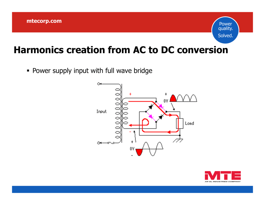
By far the majority of today’s non-linear loads are rectifiers with DC smoothing capacitors. These rectifiers typically come in 3 types – (i) single phase, line-to-neutral, (ii) single phase, phase-to-phase and (iii) three-phase.
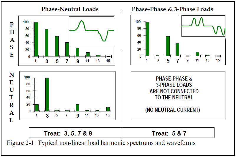
Single-phase line-to-neutral rectifier loads, such as switch-mode power supplies in computer equipment, generate current harmonics 3rd, 5th, 7th, 9th and higher. The 3rd will be the most predominant and typically the most troublesome. 3rd, 9th and other odd multiples of the 3rd harmonic are often referred to as triplen harmonics and because they add arithmetically in the neutral are also considered zero sequence currents. Line-to-neutral non-linear loads can be found in computer data centers, telecom rooms, broadcasting studios, schools, financial institutions, etc.
208V single-phase rectifier loads can also produce 3rd, 5th, 7th, 9th and higher harmonic currents but if they are reasonably balanced across the 3 phases, the amplitude of 3rd and 9th will be small. Because they are connected line-line, these loads cannot contribute to the neutral current. The largest current and voltage harmonics will generally be the 5th followed by the 7th. Typical single phase, 208V rectifier loads include the switch-mode power supplies in computer equipment and peripherals.
Three-phase rectifier loads are inherently balanced and therefore generally produce very little 3rd and 9th harmonic currents unless their voltage supply is unbalanced. Their principle harmonics are the 5th and 7th with 11th and 13th also present. They cannot produce neutral current because they are not connected to the neutral conductor. The rectifiers of variable speed drives and Uninterruptible Power Supplies (UPS) are typical examples of three-phase rectifier loads.
Figure 2-1: Typical non-linear load harmonic spectrums and waveforms
Harmonics and Harmonic Mitigating Transformers (HMT’s) Questions and Answers
This document has been written to provide answers to the more frequently asked questions we have received regarding harmonics and the Harmonic Mitigating Transformer technology used to address them. This information will be of interest to both those experienced in harmonic mitigation techniques and those new to the problem of harmonics. For additional information visit our Website at www.mirusinternational.com.
Published by Carelabs (Carelabz), Website: carelabz.com
Image: Carelabz
Load Flow Analysis / Power Flow Analysis
Power systems across the world subjected to great demands owing to expansions in the networks. Rapid development of a nation in every sphere is interlinked with its power transmission capacity. This can be done by adding new lines and by upgrading existing ones by adding new devices like FACTS. A stable power transmission network ensures prosperity.
Voltage instability in any network may lead to system collapse, when the bus voltage drops to such a level from which it cannot recover. In such a situation, complete system blackouts may take place. Hence voltage stability analysis is very important for successful process and planning of power system and for decreasing system losses. In this context, Load Flow or Power Flow Study and Analysis has been found useful by researchers in Voltage Stability Studies and Contingency Analysis.
Voltage Stability
Voltage stability is capacity of a power system to manage acceptable voltages at all buses in the system under normal conditions and after subjected to Voltage instability results in voltage collapse. Voltage collapse is the process by which the voltage falls to a low, unacceptable value as a result of an avalanche of events accompanying voltage instability. Voltage failure usually appears in power systems which usually heavy loaded failure and has reactive power shortages. In recent years voltage instability has attracted attention of power system planning and operating engineers as well as researchers. This is due to the frequent voltage collapses occurring in different parts of the world. Therefore Voltage Stability Analysis is important for researchers and power system planners to prevent such incidents from occurring.
Voltage Stability Analysis
The different methods used are:
P-V curve method.
V-Q curve method and reactive power reserve.
Methods based on peculiarity of power flow Jacobean matrix at the point of voltage collapse.
Continuation power flow method.
Optimization Method
Load Flow Analysis
To begin the Voltage Stability Analysis of a power system, computation of the complex voltages at all the buses is essential. After this, power flows from a bus and the power flowing in all the transmission lines are to calculate. A computational tool for this purpose is Load Flow Analysis. This analysis helps compute the steady state voltage magnitudes at all the buses, for a particular load condition. Load flow is mainly used in planning studies, for designing a new network or expansion of an existing one. The next step would be to compare the calculated values of power flows and voltage with the steady state device limits, to estimate the health of the network
Load Flow Study
Power flow analysis is very important in planning and designing the future expansion of power systems or addition to existing ones like adding new generator sites, meeting increase load demand and locating new transmission sites.
The load flow solution yields the nodal voltages and the phase angles, the power injection, power flows and the line losses in a network.
The best place, as well as the optimal capacity of a generating station, substation and new lines can regulate by load flow study.
Minimization of System transmission losses and prevention of line overloads. The operating voltages of the buses being determined, it aids in voltage stability analysis and voltage levels at certain buses can keep within the closed tolerances. The power flow problem formulated assuming the power system network to linear, bilateral and balanced. However, the power and voltage constraints impose non-linearity in the power flow formulation and iterative techniques are essential for the solution. The different conventional techniques for solving the power flow problem are:
Gauss-Seidel (GS) Method
Newton Raphson (NR) Method
Fast Decoupled Load Flow (FDLF)
Voltage Stability and Line Compensation
One of the prime causes leading to voltage instability is reactive power imbalance in the power system network. This occurs when there is a sudden and unpredicted increase or decrease in reactive power demand in the system. Occurrence of voltage collapse can only be prevented by either reducing the reactive power load or by providing further supply of reactive power before the system reaches the point of voltage collapse. During situations of outage in some critical lines, the generators are capable of supplying limited reactive power. But in the process, the real powers of the generators compromised while supplying this reactive power. In long transmission lines, the line length and the degree of shunt compensation are the most important factors affecting the power frequency voltages under normal and fault conditions. An open-end or unloaded line experiences a rise in the receiving end voltage related to sinusoidal input voltage, known as Ferranti effect. On the other hand, an overloaded line experiences a sequential reduction in voltage leading to voltage collapse at the weakest bus. To stabilize the line voltage, reactive power (VAR) compensation required, which is control of reactive power to enhance power system network performance. The two important features of reactive power compensation are:
Load Compensation and
Voltage Support.
The aim of voltage support is to decrease the voltage variations at a given terminal of a transmission line.
Line inductance compensation done by sequence capacitors and the line capacitance to earth by shunt reactors. Optimal placement of sequence capacitors are at different places along the line, when that of the shunt reactors is in the stations at the end of the line. In this way, the voltage drop/rise between the ends of the line can decrease both in amplitude and phase angle.
Published by Mirus International Inc., [2010-01-08] MIRUS-FAQ001-B2, FAQ’s Harmonic Mitigating Transformers, 31 Sun Pac Blvd., Brampton, Ontario, Canada. L6S 5P6.
A load is considered non-linear if its impedance changes with the applied voltage. The changing impedance means that the current drawn by the non-linear load will not be sinusoidal even when it is connected to a sinusoidal voltage. These non-sinusoidal currents contain harmonic currents that interact with the impedance of the power distribution system to create voltage distortion that can affect both the distribution system equipment and the loads connected to it.
In the past, non-linear loads were primarily found in heavy industrial applications such as arc furnaces, large variable frequency drives (VFD), heavy rectifiers for electrolytic refining, etc. The harmonics they generated were typically localized and often addressed by knowledgeable experts.
Times have changed. Harmonic problems are now common in not only industrial applications but in commercial buildings as well. This is due primarily to new power conversion technologies, such as the Switch-mode Power Supply (SMPS), which can be found in virtually every power electronic device (computers, servers, monitors, printers, photocopiers, telecom systems, broadcasting equipment, banking machines, etc.). The SMPS is an excellent power supply, but it is also a highly non-linear load. Their proliferation has made them a substantial portion of the total load in most commercial buildings.
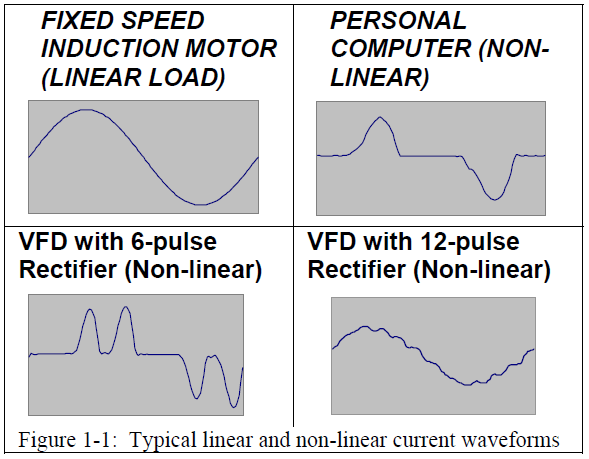
Examples of the current drawn by various types of equipment are shown in Figure 1-1. The most common form of distorted current is a pulse waveform with a high crest factor. The SMPS is one such load since it consists of a 2-pulse rectifier bridge (to convert AC to DC) and a large filter capacitor on its DC bus. The SMPS draws current in short, high-amplitude pulses that occur right at the positive and negative peaks of the voltage. Typically these high current pulses will cause clipping or flat-topping of the 120VAC supply voltage. The “double-hump” current waveform of the 6-pulse rectifier in a UPS or a VFD also will cause clipping or flat-topping of the 480V or 600V distribution system.
Figure 1-1: Typical linear and non-linear current waveforms
Harmonics and Harmonic Mitigating Transformers (HMT’s) Questions and Answers
This document has been written to provide answers to the more frequently asked questions we have received regarding harmonics and the Harmonic Mitigating Transformer technology used to address them. This information will be of interest to both those experienced in harmonic mitigation techniques and those new to the problem of harmonics. For additional information visit our Website at www.mirusinternational.com.
Published by Carelabs (Carelabz), Website: carelabz.com
Image: Carelabz
A Short circuit analysis is used to determine the magnitude of short circuit current, the system is capable of producing, and compares that magnitude with the interrupting rating of the overcurrent protective devices (OCPD). Since the interrupting ratings are based by the standards, the methods used in conducting a short circuit analysis must conform to the procedures which the standard making organizations specify for this purpose. The American National Standards Institute (ANSI) publishes both the standards for equipment and the application guides, which describes the calculation methods.
Short-Circuit Currents are currents that introduce large amounts of destructive energy in the forms of heat and magnetic force into a power system. A short circuit is sometimes called a fault. It is a specific kind of current that introduces a large amount of energy into a power system. It can be in the form of heat or in the form of magnetic force. Basically, it is a low-resistance path of energy that skips part of a circuit and causes the bypassed part of the circuit to stop working. The reliability and safety of electric power distribution systems depend on accurate and thorough knowledge of short-circuit fault currents that can be present, and on the ability of protective devices to satisfactorily interrupt these currents. Knowledge of the computational methods of power system analysis is essential to engineers responsible for planning, design, operation, and troubleshooting of distribution systems.
Short circuit currents impose the most serious general hazard to power distribution system components and are the prime concerns in developing and applying protection systems. Fortunately, short circuit currents are relatively easy to calculate. The application of three or four fundamental concepts of circuit analysis will derive the basic nature of short circuit currents. These concepts will be stated and utilized in a step-by step development.
The three phase bolted short circuit currents are the basic reference quantities in a system study. In all cases, knowledge of the three phase bolted fault value is wanted and needs to be singled out for independent treatment. This will set the pattern to be used in other cases.
A device that interrupts short circuit current, is a device connected into an electric circuit to provide protection against excessive damage when a short circuit occurs. It provides this protection by automatically interrupting the large value of current flow, so the device should be rated to interrupt and stop the flow of fault current without damage to the overcurrent protection device. The OCPD will also provide automatic interruption of overload currents.
Short-circuit calculations are required for the application and coordination of protective relays and the rating of equipment. All fault types can be simulated. Carelab’s short-circuit study provides a detailed report identifying breaker ratings, breaker fault duties, discussions, and recommendations for any deficiencies found
Risks Associated With Short Circuit Currents
The building/facility may not be properly protected against short-circuit currents. These currents can damage or deteriorate equipment. Improperly protected short-circuit currents can injure or kill maintenance personnel. Recently, new initiatives have been taken to require facilities to properly identify these dangerous points within the power distribution of the facility.
Why Is A Short Circuit Dangerous?
A short circuit current can be very large. If unusually high currents exceed the capability of protective devices (fuses, circuit breakers, etc.) it can result in large, rapid releases of energy in the form of heat, intense magnetic fields, and even potentially as explosions known as an arc blast. The heat can damage or destroy wiring insulation and electrical components. An arc blast produces a shock wave that may carry vaporized or molten metal, and can be fatal to unprotected people who are close by.
Fault current calculations are necessary to properly select the type, interrupting rating, and tripping characteristics of power and lighting system circuit breakers and fuses. Results of the fault current calculations are also used to determine the required short-circuit ratings of power distribution system components including bus transfer switches, variable speed drives, switchboards, load centres, and panel boards. In calculating the maximum fault current, it is necessary to determine the total contribution from all generators that may be paralleled and the motor contribution from induction and synchronous motors.
Short Circuit Analysis is performed to determine the currents that flow in a power system under fault conditions. If the short circuit capacity of the system exceeds the capacity of the protective device, a dangerous situation exists. Since growth of a power system often results in increased available short-circuit current, the momentary and interrupting rating of new and existing equipment on the system must be checked to ensure the equipment can withstand the short-circuit energy (see Device Evaluation). Fault contributions for utility sources, motors and generators are taken into consideration.
A Short Circuit Analysis will help to ensure that personnel and equipment are protected by establishing proper interrupting ratings of protective devices (circuit breaker and fuses). If an electrical fault exceeds the interrupting rating of the protective device, the consequences can be devastating. It can be a serious threat to human life and is capable of causing injury, extensive equipment damage, and costly downtime.
On large systems, short circuit analysis is required to determine both the switchgear ratings and the relay settings. No substation equipment can be installed with knowledge of the complete short circuit values for the entire power distribution system. The short circuit calculations must be maintained and periodically updated to protect the equipment and CC the lives. It is not safe to assume that new equipment is properly rated.
The results of a Short Circuit Analysis are also used to selectively coordinate electrical protective devices.
What is Short Circuit Analysis?
Short circuit analysis essentially consists of determining the steady state solution of a linear network with balanced three phase excitation. Such an analysis provides currents and voltages in a power system during the faulted condition. This information is needed to determine the required interrupting capacity of the circuit breakers and to design proper relaying system. To get enough information, different types of faults are simulated at different locations and the study is repeated. Normally in the short circuit analysis, all the shunt parameters like loads, lime charging admittances are neglected* Then the linear network that has to be solved comprises of
Transmission network
Generator system and
Fault. By properly combining the representations of these components we can solve the short circuit problem
Carelabs allows you to perform a per unit calculation on any system you are working with. We automatically converts the entire system (panel boards, transformers, generators, motorized items and cables) into a unique impedance unit from which you can obtain the rating of the short circuit current at any given point. The process is simple, efficient and will save you both money and time.
Carelabs provides short-circuit calculations for single and multiple faults, together with a number of reporting options. As short-circuit calculations are needed for a variety of purposes, the short-circuit calculation in Carelabs supports different representations and calculation methods based on a range of international standards, as well as the superposition method (also known as the Complete Method).
What Are Bolted, Arcing and Ground Faults?
A bolted fault typically results from a manufacturing or assembly error that results in two conductors of different voltages being “bolted” together, or a source of power being directly connected (bolted) to ground. Since the connectors are solidly bolted there in no arc created and the high current quickly trips a protective device limiting the damage.
An arc fault is one in which the short circuit creates an arc. An arc is a flow of electricity between two conductors that are not in contact. The resulting intense heat can result in a fire, significant damage to the equipment, and possibly an arc flash or arc blast resulting in serious injuries.
A ground fault is when electricity finds an unintended, low resistance, path to ground. When that path goes through a human body the resulting heat can cause serious burns, and the electrical shock can disrupt the functioning of the human heart (fibrillation).
What Are Symmetrical and Asymmetrical Currents?
A polyphase system may experience either a symmetrical or an asymmetrical fault. A symmetrical fault current is one that affects all phases equally. If just some of the phases are affected, or the phases are affected unequally, then the fault current is asymmetrical.
Symmetrical faults are relatively simple to analyse, however they account for very few actual faults. Only about 5% of faults are symmetrical. Asymmetrical faults are more difficult to analyse, but they are the more common type of fault.
What Are Protective Devices for Short Circuit Analysis?
Protective devices are designed to detect a fault condition and shut off the electric current before there is significant damage. There are a number of different types of protective devices, the two most common are:
Fuses and Circuit Breakers
Fuses and circuit breakers are used to protect an electrical circuit from an over-current situation, usually resulting from a short circuit, by cutting off the power supply. Fuses can only be used once. Circuit breakers may be reset and used multiple times.
Ground Fault Interrupter (GFI)
This is a device that detects when the current flow in the energized conductor does not equal the return current in the neutral conductor. The GFI protects people by quickly cutting off the current flow preventing injuries resulting from shock. Ground Fault Interrupters are typically used in homes for bathroom, kitchen, and outdoor electrical sockets. The GFI will typically be built into the electrical socket.
A GFI does not provide over-current protection, and the circuit that includes a GFI will also include a fuse or circuit breaker.
In addition to fuses, circuit breakers, and GFIs, there are electrical protection devices that:
detect changes in current or voltage levels
monitor the ratio of voltage to current
provide over-voltage protection
provide under-voltage protection
detect reverse-current flow
detect phase reversal
When are Short Circuit Analysis Needed?
The first short-circuit analysis should be performed when a power system is originally designed, though this should not be the only time. These studies need to occur with any facility expansion or with the addition of any new electrical equipment such as circuit breakers or new transformers and cables. Without any new additions or changes, short circuit studies still need to occur on a regular basis of at least every 5-6 years.
How Is Short Circuit Current Calculated?
Short-circuit calculations are required to correctly apply equipment in accordance with NEC, and ANSI standards. Depending on the size and utility connection, the amount of detail required to perform these calculations can vary greatly. Carelabs short-circuit analysis will include calculations performed in accordance with the latest ANSI standards.
Switches, fuses, and breakers that need to interrupt or close into a fault are of special concern. Cables and buswork also have short-circuit withstand limitations, and a thorough study will examine non-interrupting equipment, as well as switches and breakers. Standards such as ANSI C37.010 and C37.13 outline the recognized calculation methods for these equipment-rating analyses.
These short circuit studies are performed using power system software as per IEEE standards. For larger systems, these short circuit calculations to be performed for both switch gear ratings and relay settings. Knowledge of the computational methods of power system analysis is essential to engineers responsible for planning, design, operation, and troubleshooting of distribution systems. A short-circuit study is an analysis of an electrical system that determines the magnitude of the currents that flow during an electrical fault. Comparing these calculated values against the equipment ratings is the first step to ensuring that the power system is safely protected. Once the expected short-circuit currents are known, a protection coordination study is performed to determine the optimum characteristics, ratings and settings of the power system protective devices.
NEC 110 requires that a short circuit analysis be done for all electrical equipment and panels. The two most common standards for short circuit current calculations are the ANSI/IEEE C37.010-1979 standard and the International Electro-technical Commission (IEC) 60909 standard.
The ANSI C37.010 standard was intended to be used for power circuit breaker selection, but it does provide the information needed for NEC 110 required labelling. The IEC 60909-3:2009 standard is more generic. It is intended to provide general guidelines for short-circuit analysis of any asymmetrical short circuit in a three-phase 50 Hz or 60Hz A.C. electrical system.
Either the ANSI or the IEC short circuit calculation method can be used. They have been compared and found to produce similar results. The ANSI method is commonly used in short circuit current calculation software.
Our short circuit analysis service:
Is done with support of IEC 60909 (including 2016 edition), IEEE 141/ANSI C37, VDE 0102/0103, G74 and IEC 61363 norms and methods
Is calculation of short-circuit currents in DC grids according to IEC 61660 and ANSI/IEEE 946
We do complete superposition method, including dynamic voltage support of generators connected via power electronics
Multiple fault analysis of any kind of fault incl. single-phase interruption, inter-circuit faults, fault sweep along lines, etc.
Diakoptic Model For The Short Circuit Analysis (Do We Use This?)
In the short circuit analysis, it is customary to neglect the loads and other shunt parameters to the ground. Under this condition, impedance representation for the transmission network with ground as reference does not exist. However, connection to the ground is established at the generator buses, representing the generator as a constant voltage source behind appropriate reactant. Hence let us consider the combined transmission-generator network and while tearing the network, let us ensure that each sub-network has at least one generator. In practice this should pose no difficulty since large power system 84 networks normally consist of different areas having generations in each area.
Neplan
Short circuit analysis is performed so that existing and new equipment ratings were sufficient to with stand the available short circuit current. This short circuit analysis can be done either through hand calculations or through known software like NEPLAN.
Using NEPLAN we can perform short circuit studies on electrical systems in a quick time and effective manner in four steps.
Data Collection and SLD Preparation
Short circuit calculations
Relay Coordination Studies
Load flow Analysis
Why chose Carelabs for Short Circuit Analysis?
At Carelabs we differ from competitors in our size and structure and this allows us to be more responsive to change. It also allows us to provide personalized and superior services to you. We follow NFPA-70E and IEEE 1584 guidelines in order to guarantee that we always meet the highest industry standards.
Benefits of Short Circuit Analysis
Conducting a short circuit analysis has the following benefits:
Helps avoid unplanned outages and downtime
Is critical for avoiding interruptions of essential services
Reduces the risk of equipment damage and fires
Increases safety and protects people from injuries
Determines the level and type of protective devices that are needed
Provides the information needed for NEC and NFPA required labels
Keeps you in compliance with NEC requirements
Reduces the risk a facility could face and help avoid catastrophic losses
Increases the safety and reliability of the power system and related equipment