Some Comments on Power Acceptability Curves

Published by

• G. Heydt , Arizona State University Tempe, Arizona USA
• R. Thallam, Salt River Project Phoenix, Arizona USA
• M. Albu, Universitatea Politehnica Bucureşti Bucharest, Romania

CARIBBEAN COLLOQUIUM ON POWER QUALITY (CCPQ), JUNE 2003

---

Abstract

Power acceptability curves, also known as voltage vulnerability or sensitivity curves, have been used for over 30 years to characterize momentary events of low voltage in power distribution systems. In this paper, a summary of how the curves were developed is given, and some thoughts on the applicability of the curves are presented.

Index terms: CBEMA curve, voltage sags, power quality, power acceptability, voltage sensitivity.

I. Power acceptability

Many power quality indices relate to steady state phenomena, and relatively few relate to momentary events. However, many power quality engineers feel that bus voltage sags, a natural consequence of a highly interconnected transmission system, may be the most important type of power quality degradation, and therefore a useful measure of the severity of these events is desirable. One such metric is the power acceptability curve (or voltage sensitivity or voltage vulnerability curve) which is a graphic metric of the severity of bus voltage sags plotted versus the duration of these events. Table I shows some of the issues that might be captured by a power acceptability (sensitivity) metric.

The best known of the graphical metrics for bus voltage sensitivity is the Computer Business Equipment Manufacturing Association (CBEMA) curve which is a graphic depicting the severity of a distribution bus voltage sag, Δ V, versus its duration T. The Δ V-T plane is a two dimensional space in which the line Δ V = 0 represents the case that distribution voltage is at rated value, and the Δ V < 0 half-plane is the bus voltage sag region. Overvoltage and undervoltage events of very minimal impact (small | Δ V | ) are considered ‘acceptable’ in the sense that loads are not disrupted; further, very short duration events (small T) are considered acceptable. Thus the Δ V – T plane is divided into acceptable and unacceptable regions. Fig. (1) shows the CBEMA power acceptability curve. The CBEMA curve depicted in Fig. (1) has Δ V indicated as a percent of rated voltage, and T shown on a logarithmic scale in seconds.

Table I Some issues in voltage sag and overvoltage events in primary distribution systems

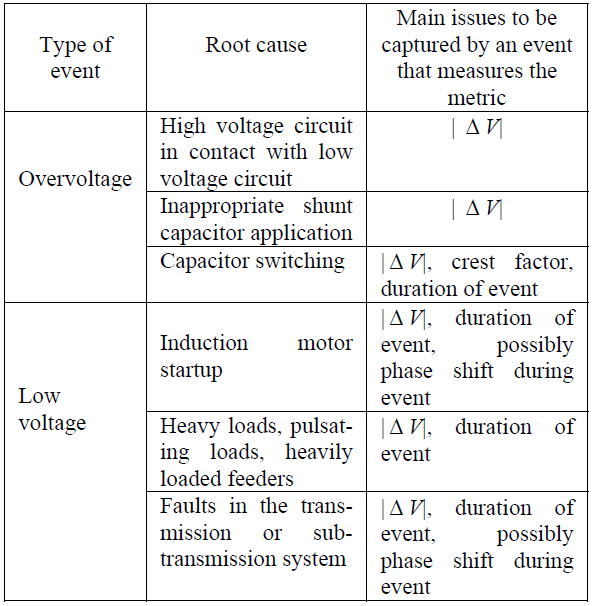
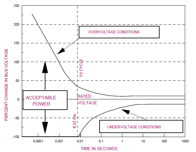
Fig. (1) The CBEMA power acceptability curve

References [1-3] discuss a fuzzy logic alternative to assess voltage – load sensitivity, testing of loads to CBEMA standards, and computer performance during voltage sags respectively. Bollen has discussed a classification system of voltage sags and their effects [4]. Ride through issues for adjustable speed drives appear in [5]. References [6] and [7] by Kyei and other researcher describe research into the ‘derivation’ of these curves by using data from appropriate models of loads.

It is evident that power acceptability curves have frailties in design and application. For example, very short duration events (e.g., less than a cycle in duration) have an ambiguity in the sense that the duration of the event may be difficult to identify, and the point on- wave of the disturbance may have significant impact on the load. Point-on-wave information is not depicted in the Δ V-T plane. Further, the three phase implications of a power acceptability curve as indicated above are not clear: should one utilize phase information in the Δ V-T plane, or the positive sequence of the distribution voltage? Or is the graph basically a single phase representation? Another commonly asked question relates to the equation of the loci shown in Fig. (1). The CBEMA curve was developed from experimental and historical data: that is, cases of load disruption of mainframe computers were plotted in the Δ V-T plane, and a separator was developed to identify the acceptable and unacceptable regions.

II. A power quality standard

In 1998, Ayyanar and others [7] suggested the concept of a standard to represent whether power distributed is acceptable or unacceptable. The essence of the concept is that one needs to write a concrete criterion upon which acceptability is decided. One ultimate criterion of power acceptability relates to the operating status of the industrial process.

The particular power quality criterion depends on the nature of the load. For example, simple incandescent lighting loads may have a very loose criterion for acceptability, while certain sensitive computer controls may have a much more restrictive criterion. The difficulty in the selection of a single suitable criterion is confounded by the many possible load types. For simplicity, consider the rectifier load type depicted in Fig. (2). Voltage sags occur due to faults in the transmission, subtransmission, and primary distribution system, and they appear as low voltage conditions at V_ac depicted in Fig. (2). If the sag is of short duration and shallow depth, the ultimate industrial process ‘rides through’ the disturbance. This means that although V_ac is depressed, V_dc does not experience a sufficient disturbance to affect the load. The concept of a voltage standard is introduced at this point: a voltage standard is a criterion for power acceptability based on a minimum acceptable DC voltage at the output of a rectifier below which proper operation of the load is disrupted.

As an example of a voltage standard consider the following: if V_dc drops below 87% of rated voltage, the load is lost, and the distribution power is deemed to be unacceptable. The term ‘standard’ used in this context refers to the ultimate criterion upon which a decision of acceptability of supply is made. The use of the term ‘standard’ is not meant to imply an industry wide standard such as an IEEE standard. Fig. (3) shows a simulation study suitable for quantifying the effect of sags on rectifier load performance.

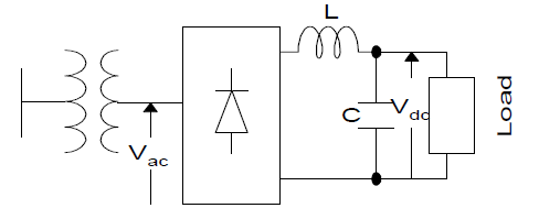
Fig. (2) A rectifier load

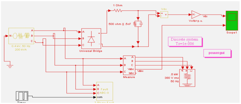
Fig. (3) Simulation of a three phase rectifier load

III. Analytical synthesis of the CBEMA curve

The CBEMA curve was derived from experimental and historical data taken from mainframe computers. The best engineering interpretation of the CBEMA curve can be given in terms of a voltage standard applied to the DC bus voltage of a rectifier load. Consider the case of either a single phase full wave bridge rectifier or the three phase bridge counterpart. Let the load on the DC side be an RLC load. If the DC bus voltage under a faulted condition is plotted as a function of the sag duration, the resulting curve is depicted in Fig. (4). From Fig. (4), the locus of V_dc could be represented as a double exponential in the form,

V_dc(t) = A + Be^–bt + C e^-ct.

Parameter A is the ultimate (t → ∞ ) voltage, V_end, of the rectifier output. For the single phase case, and for the balanced three phase case, A is simply the depth of the AC bus voltage sag.

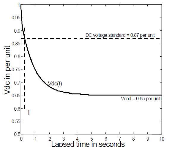
Fig. (4) Locus of V_dc(t) under fault conditions (at t = 0) for a single phase bridge rectifier

For more complex cases, e.g. unbalanced sags, parameter A can similarly be identified as the ultimate DC circuit voltage if the sag were to persist indefinitely (this is readily calculable by steady state analysis of the given sag condition and the rectifier type). If three points are selected on the CBEMA curve to identify the RLC filter combination used in the rectifier types considered in the original CBEMA tests, one finds,

V_dc(t) = V_end + 0.288e^-1.06t + (0.712-V_end)e^-23.7t. (1)

As an example, let the voltage standard be V_dc ≥ 0.87. Then the V_dc excursion becomes unacceptable at T when V_dc = 0.87 in Equation (1). Solution for Vend in terms of t = T in this expression gives

---

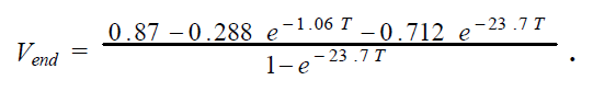
This is the formula for the undervoltage limb of the CBEMA curve (V_end in per unit, T in seconds).

IV. Some practical considerations

Application of the CBEMA curve or most other power quality ‘standards’ require certain practical considerations. Among these non-ideal considerations are:

• The meaning of Δ V for short term events, especially when represented in root-mean square (RMS) values
• Three phase considerations
• Non ideal sags (e.g., the sag is –10% for the first few cycles, followed by –15% for the next few cycles – or even less ideal conditions in which the sag has no well defined value
• Repeating events (e.g., one event, followed by restoration of normal operating conditions, followed by another event)
• Point-on wave issues (see Section 5)
• Multiple loads each with different sensitivity to bus voltage magnitude

Some of these issues are more easily considered than others. However, the rectifier and 87% V_dc interpretation given above do apply in all the cited practical cases. That is, at least in theory, a given non ideal, and perhaps three phase case, could be simulated utilizing a rectifier load with a DC circuit filter of the type cited above in connection with the ‘derivation of the CBEMA curve’. The three phase case is most easily considered as follows: Fig. (4) shows a power acceptability curve for a three phase rectifier. The case considered here is that of a phase A to ground fault using an 87% V_dc voltage standard. The procedure for the development of the power acceptability curve is similar to the one employed in deriving Equation (1). The unbalanced rectifier is analyzed simply, and V_dc(t) in this case is given as

V_dc(t) = V_end + 0.159e^-0.158t + (0.841-V_end)e^-4.63t . (2)

In Equation (2), the time constants were obtained using an LC filter on the DC side of a three phase, six-pulse bridge rectifier. The values of the LC were chosen to agree with the filter design used in the single phase case mentioned in connection with the derivation of Equation (1). That is, the CBEMA curve was found to correspond to the single phase rectifier case plus filter F. If filter F is used as a filter in the three phase case, Equation (2) results. Select a voltage standard of V_dc ≥ 0.87 When substituted into Equation (2) gives a formula for the power acceptability curve shown in Fig. (5) as

---

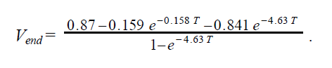
Other unbalanced faults are analyzed similarly.

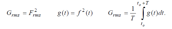
The issue of short term representation of Δ V in terms of RMS values was considered in [8]. In many power quality studies, waveforms are characterized through a RMS value,

---

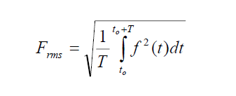
where f(t) is a time signal and T is either the period of the time signal or a suitably long time.

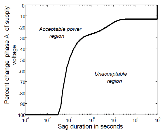
Fig. (5) Power acceptability curve for a three phase rectifier load with a phase-ground fault at phase A, 87% V_dc voltage standard

For the periodic case, when T is an integer multiple of the period of f(t), and t₀ is a fixed point on the wave, the RMS value is termed a synchronous RMS (s-RMS). The s-RMS operation maps a time signal to a single point and can be visualized as an information concentrator. It is a simple matter to demonstrate that the s-RMS quantifies the Joule effect of a sinusoidal voltage or current. Reference [9] contains a discussion of applications and calculation procedures. Fig. (6) shows an example of a short term voltage sag for which the following key parameters are noted:

• T_w is the length of the observation time window
• T_s is the duration of the change in signal’s amplitude
• T is the period of the signal, assumed as with sinusoidal variation
• T₀ is the moment of the amplitude change (considering that the observation window starts at t = 0)
• r is the magnitude of amplitude change (in p.u.; the reference value is the amplitude at t < t₀). Note that r ≤ 1 and r ≥ 0 for voltage sags, r < 0 for swells.
• ϕ is the phase at t = 0.

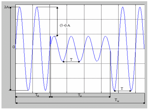
Fig. (6) Model of a voltage sag signal

In power quality studies, the effects on consumers are often quantified in terms of the deviation of secondary distribution voltage RMS values. However when sag events are of short duration, the RMS values may have a problematic interpretation. There are many hardware and software algorithms which compute RMS values, and it becomes advisable to identify the hidden possible errors in calculation and interpretation. Note that the RMS operator is nonlinear, but working with F²_rms and f²(t) gives the linear formulation,

---

If the RMS operator is continuously carried out over a windowed time T, using past samples from the input signal g(t), a moving average finite impulse response filtering is performed,

---

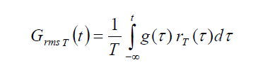
where r_T(t) is a rectangular pulse which is zero everywhere except in the interval [t–T, t] where it is unity. In the Fourier domain

---

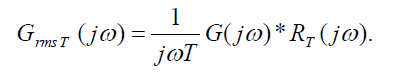
The notation (*) denotes frequency domain convolution. Equation (4) indicates that there is a frequency response interpretation to the RMS operator. References [10,11] further discuss factors relating to the calculation of the RMS value.

The problem of repeated events is considered in [12]. The concept of repeated events is problematic because a second event, following closely after a first event, could have greater impact than an isolated event that is identical to the cited second event. For example, a momentary sag occurring at t = 0, for six cycles, followed by a second event at t = 0.15 s (60 Hz system) of duration six cycles might be analyzed; in such a case, the analysis of the second event of six cycles is quite different from an analysis performed of an isolated, non-repeated event of identical duration and sag depth. Heydt [12] suggests that there is a recovery time for which a system must progress in order to render an event in isolation from previous events. The concept of a recovery time is very similar to that of the ‘derivation of the CBEMA curve’ given above: that is, the recovery time of a sag can be plotted in the form of isopleths on a Δ V-T plane. The alternative, if the information is available, is to simulate the double (or triple, or multiple) event using a circuit as indicated in Figures (2) and (3).

The issues of multiple loads can be depicted as Fig. (7). For such a configuration, the CBEMA curve for each load may be calculated, tailoring the curve as needed. When the resultant CBEMA curves are drawn on a common Δ V-T plane, the inner area contains the acceptable region, and the outer area is the unacceptable region as shown in Fig. (8). The area(s) between the inner and outer regions represent power acceptable to some loads, and unacceptable to others.

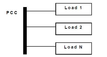
Fig. (7) Multiple loads at a point of common coupling (PCC)

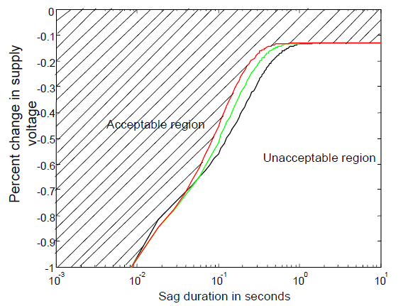
Fig. (8) Power acceptability region for the case of multiple loads

V. Point on wave issues

A momentary interruption of voltage or momentary sag in voltage magnitude may initiate at any point in the sinusoidal cycle as indicated in Fig. (9). For a linear load at unity power factor, the load current will be identical in phase to the indicated voltage. The energy transfer from the source to the load depends generally on θ_o as well as the duration of the sag. Consider a total outage of supply voltage. Integrating v(t)i(t) over θ_o to θ_o + θ where θ is the duration of the sag represented in radians assuming 60 Hz (or 50 Hz as appropriate), one finds that the energy that should have been delivered during the sag (and is now unserved due to the outage) is W,

---

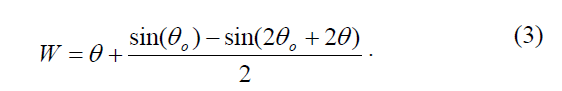
For this simple formula, the rms supply voltage and current are both 1.0 per unit. Note that for values of θ that correspond to less than a half cycle (i.e., θ < π ), the CBEMA curve dictates that power delivery is ‘acceptable’. For longer duration outages, W depends not only on the duration of the outage θ , but also the point on wave θ_o at the initiation of the sag.

The more general case of a linear load with power factor cos(ϕ ) is more involved since the instantaneous power is a double frequency sine wave whose DC offset (i.e., the average power) is proportional to cos(ϕ ) . The unserved energy on total outage is

---

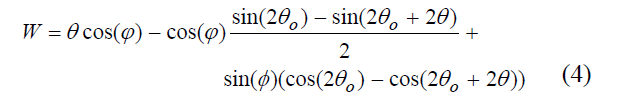
Collins and others have discussed the practical implications of the point on wave of the initiation of a voltage sag, including laboratory verified phenomena [13]. For long outages (largeθ , e.g., much larger than three cycles or 6π radians), the term in Equations (3) and (4) that is proportional to θ dominates, and the unserved energy is no longer greatly dependent on the point on wave at the sag initiation.

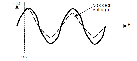
Fig. (9) Point on wave initiation of a voltage sag event

VI. A single index to show compliance with CBEMA

In most areas of engineering, it is important to use indices to measure or quantify the quality of performance. Power acceptability curves graphically depict power quality; but is there an index that can be used to assess “acceptability” or “unacceptability”? Consider Fig. (10) in this matter. Point P represents an event Δ V = Δ V_p and T = T_p (shown as ‘unacceptable’ in Fig. (10)). As an index of power acceptability, it is proposed to vary the threshold V_T until the power acceptability curve passes through P. This is shown as dashed lines in Fig. (10). Then, one sets V_T to V_Tp ,

---

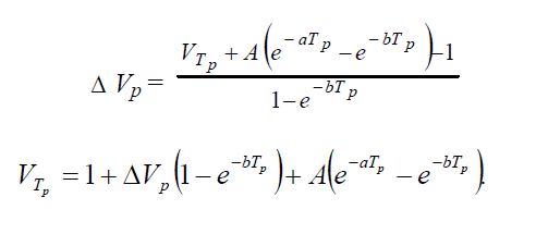
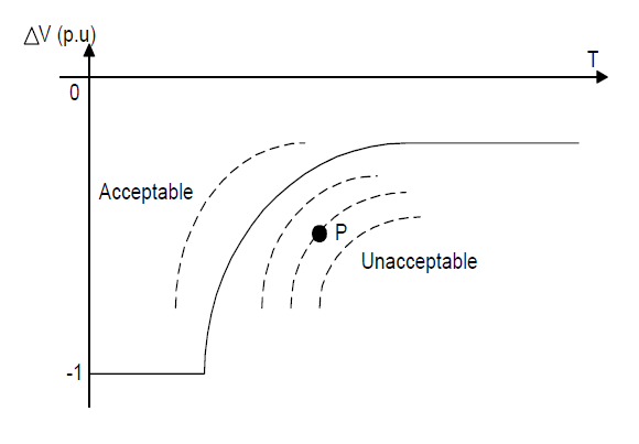
Fig. (10) Graphic interpretation of an index of power acceptability for an event P

Consider the index V_Tp / VT . If V_Tp / V_T ≥ 1, the point P represents an acceptable event. It is a simple matter to show that the theoretical maximum of the index V_Tp / V_T is 1/V_T . Introduce the notation I_pa for the new index,

I_pa = V_Tp / V_T.

If one uses the notation T_x as the maximum time for which acceptable power is attained upon a total outage (i.e., Δ V = -1),

---

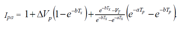
This is an index of power acceptability for the event P. When the index is greater than unity, one is in the acceptable power region, and when the index is below unity, one is in the unacceptable region. At unity itself, the event is exactly on the CBEMA curve.

VII. Recommendations and concluding comments

In this paper, the CBEMA curve was revisited and the curve was analytically synthesized using a new concept, the voltage standard. The standard refers to an ultimate criterion that power is unacceptable if the DC voltage of a certain rectifier load drops below 87% of rated value. A double exponential equation describing the CBEMA curve is developed. This provides a useful method to consider the effect of unbalanced voltage sags and to develop CBEMA-like curves for other types of loads. A scalar index of compliance termed I_pa has been illustrated. This index is based on the CBEMA curve compliance.

Additional practical considerations relating to power acceptability include:

• The meaning of Δ V for short term events, especially when represented in root-mean square (RMS) values
• Three phase considerations
• Non ideal sags
• Repeating events
• The energy served to a load during a sag as a function of the point-on-wave of the initiation of the event
• Multiple loads each with different sensitivity to bus voltage magnitude.

It appears that the main advantage of the CBEMA curve is the ease in application, and also in the familiarity of the concept by most power engineers.

Although accuracy of the curve in predicting true acceptability – unacceptability of the power supply may not be a strong point of CBEMA technology, at least some problematic issues of its application may be resolved using the concept of a voltage standard.

Acknowledgements

The authors gratefully acknowledge the support of the Power Systems Engineering Research Center (PSerc) and SRP. Most of the work represented here came from Mr. John Kyei of the California ISO, Folsom CA. Dr. Raja Ayyanar of Arizona State University originated the concept of the voltage standard, and the authors acknowledge his contribution. Dr. Albu acknowledges the support of the Fullbright Fellowship.

References

[1] B. Bonatto, T. Niimura, H. Dommel, “A fuzzy logic application to represent load sensitivity to voltage sags,” Proceedings International Conference on Harmonics and Quality of Power, October, 1998, pp. 60-64.
[2] E. Collins, R. Morgan, “A three phase sag generator for testing industrial equipment,” IEEE Transactions on Power Delivery, v. 11, No. 1, January, 1996, pp. 526 – 532.
[3] D. Koval, “Computer performance degradation due to their susceptibility to power supply disturbances,” Conference Record, IEEE Industry Applications Society Annual Meeting, October, 1989, v. 2, pp. 1754 – 1760.
[4] M. Bollen, L. Zhang, “Analysis of voltage tolerance of AC adjustable-speed drives for three-phase balanced and unbalanced sags,” IEEE Transactions on Industry Applications, v. 36, No. 3, May-June 2000, pp. 904 – 910.
[5] E. Collins, A. Mansoor, “Effects of voltage sags on AC motor drives,” Proceedings of the IEEE Technical Conference on the Textile, Fiber and Film Industry, 1997, pp. 9 – 16.
[6] J. Kyei, “Analysis and design of power acceptability curves for industrial loads,” MSEE Thesis, Arizona State University, Tempe AZ, December 2001.
[7] J. Kyei, R. Ayyanar, G. Heydt, R. Thallam, J. Blevins, “The design of power acceptability curves,” accepted for publication, IEEE Trans. on Power Delivery, 2003.
[8] M. Albu, G. Heydt, “On the use of RMS values in power quality assessment,” accepted for publication, IEEE Trans. on Power Delivery, 2003.
[9] S. Kuo, B. Lee, Real-Time Digital Signal Processing. Implementations, Applications, and Experiments with the TMS320C55X, John Wiley and Sons, New York, 2001.
[10] S. Herraiz-Jaramillo, G. Heydt, E. O’Neill-Carrillo, “Power quality indices for aperiodic voltages and currents,” IEEE Transactions on Power Delivery, v. 15, No. 2, April 2000, pp. 784 790.
[11] N. Tunaboylu, E. Collins, P. Chaney, “Voltage disturbance evaluation using the missing voltage technique,” Proceedings of the 8th International Conference on Harmonics and Quality of Power 1998, pp. 577 – 582.
[12] G. T. Heydt, Computer Analysis Methods for Power Systems, Second edition, Stars in a Circle Publications, Scottsdale, AZ, 1996.
[13] E. R. Collins, M. A. Bridgwood, “The impact of power system disturbances on AC-coil contactors,” Proceedings of the IEEE Technical Conference on the Textile, Fiber and Film Industry, 1997, pp. 2-6.