Published by Mariano Sanz, Member, IEEE, Andrés Llombart, Member, IEEE, Ángel Antonio Bayod and Joaquín Mur, Student Member, IEEE
Abstract— A new system for studying power quality (PQ) in wind turbines (WT) has been designed using a data acquisition board (DAQ), LabVIEW programming software and a portable PC. The system has been installed at wind turbines and at the power substation of a wind farm. Collected raw data are processed to get the main parameters of the system, power spectrum and dynamic response. The information obtained is completed with the data from a supply network analyser and from a data logger at the meteorological station.
Index Terms— wind energy, power quality, virtual instrument, LabView.
I. INTRODUCTION
Increasing penetration of wind energy in the supply grid makes necessary to study the power quality of the generated energy, regarding mainly three factors:
a) Voltage fluctuations and presence of harmonics in the net, due to wind gusts and due to non-natural wind oscillations caused by the presence of the tower [1].
b) Stability problems at the wind turbines due to faults in the grid [2, 3] (short circuits, lightning surges, manoeuvres, etc.), as well as the ones due to the great variability of the wind [4].
c) Wind power forecasting and optimum economical operation [5].
International Standard IEC 61400-21 has been developed to define and specify the measurement to quantify PQ of a grid connected turbine [6]. There are also available drafts of standard for characterization of PQ as IEEE P1159.1 [7] and IEC 61000-4-30 [8].
Most of the available supply network analysers do not allow neither recording of signals at high sampling rate for a long period nor complex calculus with the scanned data, needed in these studies. To achieve the samples, the Electrical Engineering Department of the University of Zaragoza has developed a measurement system that scans data from current and voltage measurement transformers. There are some sensors placed at the wind turbine speed of blades and generator, blade pitch– and at a meteorological tower [9]. The main system, composed by a portable PC, a DAQ and a signal conditioning board, is housed in a steel case to reduce interferences from nearby power systems [10].
The measuring system is completed with an additional flicker meter, that is not yet implemented in this system [11, 12], and the data logger of the meteorological station. The measures of voltage, current and harmonics have been tested in the Laboratory of Metrology of our Department.
II. THE MEASUREMENT SYSTEM
The measurement system has been installed in two wind farms with wind turbines in the 600 kW class, owned by CEASA and located in Borja and Remolinos (Zaragoza, Spain). Both farms have wound rotor asynchronous generators; Borja generators have an external variable resistor connected to their rotor (VRIG) while Remolinos ones utilise doubly fed induction generators (DFIG).
The installation located in Remolinos is composed by three systems placed at two wind turbines and at the power substation, as shown in Fig. 1. The wind velocity is taken from the meteorological station, since the measures from the anemometers placed at the rear side of the nacelle (down stream) are very noisy.

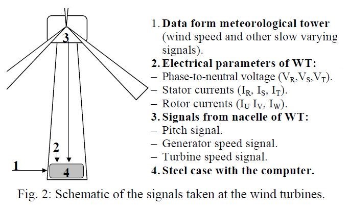
Signals that come from the top and from the ground of the wind turbines, enter the case as it is shown in Fig. 2. Measuring transformers have been used to acquire instantaneous voltage [13] and current waveforms [14]. The current transformers are of split core and voltage output (readable directly by the acquisition board). These transformers are easy of install, but they are up-to-now the main contribution to uncertainty of this system and they should be substituted.
Generator and turbine speed are measured with inductive sensors (in some WT an encoder has also been used). Signals from WT sensors are isolated and transmitted by current loop.
Wind speed is measured by means of an anemometer at meteorological tower. Propeller and cup anemometers have been employed. Propeller anemometer has quicker response, but oscillating movement of wind vane can introduce errors in turbulent winds. Other anemometers are feasible (sonic, laser, hot wire, SODAR, etc) and some of them have more precision, but they aren’t so reliable for this application and they can require temperature, humidity and pressure compensation [15, 16, 17, 18, 19].
Wind is probably the main parameter of a WT farm. However, its spatial and temporal variability make it hard to grasp. Complex orography, close obstacles as buildings or other WT, shear and tower shadow effects can affect notably to air stream that a turbine experiences [20]. Most anemometers give a punctual measure whereas it is preferable to obtain an spatial average over the swept area of a wind turbine, or even for our application, over the whole wind farm.
Nevertheless, this problem affects mainly to the estimation of economic viability of a feasible wind farm or to the control of variable speed or variable pitch WT. In order to decide whether connect at low winds or disconnect at high winds, control typically uses a cup anemometer and a wind vane placed downstream on top of the nacelle (this measure is very noisy due to turbulence, but if it is low-pass filtered, it gives enough information for this task). An option largely implemented for blade or speed control in WT is to estimate actual average wind speed from generated power and angular speed.
Due to the difficulties to get a meaningful measure of wind, it is advisable, for power quality analysis, to centre on electrical parameters of the farm instead of the wind [21].
In the first prototype, output from anemometer sensors were transmitted via current loop (4-20 mA) to the main system, where it was measured. This transmission system introduced low delay in the system (about 0,2 ms delay while time constant of typical wind sensors are around 0,5 s) and it was preferable for the study of gust. Slow varying signals, as temperature, pressure and humidity were recorded independently in a data logger. However, it resulted later that, in the analysis performed, few information was lost if all meteorological signals were centralized in the meteorological data logger. Then, data was transmitted online via EIA 485 periodically, to the computer, where they were synchronised with DAQ data. This approach makes the system more flexible and expandable.
Power supplied by DFIG is the sum of stator and rotor power. Two separated low voltage windings are utilised (see Fig. 3). Therefore, electrical measurements must be doubled since it is not typically suitable measuring high voltage inside the WT. Actually, the transformer ratio and the 690 V winding voltage has been used to compute it in 230 V, since high frequency distortion at 230 V would have required higher sampling rate or analog filtering to achieve the desired precision. Even in field measurements, some ‘True RMS’ multimeters showed 17% deviation due to inverter switching.

In VRIG located in Borja (Zaragoza, Spain), the rotor returns no power and therefore measurements are simpler. However, two current measurements are performed: stator current without capacitor compensation and total current (both in 690 V). This has allowed studying the connection and disconnection of capacitor banks installed in those WT.
Moreover, substation parameters are measured at voltage and current transformers and they served to study the effect of a number of turbines in the point of common coupling (PCC). On one hand, the effect of starting, stopping and power oscillations (due mainly to tower shadow and wind shear) is more easily studied locally at a single WT. On the other hand, the global effect of all WT should be analysed at the output of the wind farm (statistical dispersion of events and partial compensation of fluctuations play a key role in the overall behaviour of the system) [22].
III. ACQUISITION AND ANALYSIS SOFTWARE
A set of computer programs has been designed to match the requirements of several types of analysis. The system has been used in several locations, so when the acquisition program is started, it asks the user the measuring location to adjust the system configuration.
Integrating period has been adjusted depending on the type of analysis. Wind gust response and starting and stopping cases need recording current and voltage waveforms with a high sampling rate (3.000 Hz minimum according to IEC 61400-21 and from 1.600 to 6.400 Hz for 50 Hz grid according to IEEE P1159.1, depending on the PQ event), whereas power curve from manufacturer is calculated based on 10 minutes average, according to IEC 61400-12 [23]. The acquisition software can work in two modes:
- Digital oscilloscope recorder. The system stores the waveform of all inputs. Afterwards, data are stored in CD-ROM and numeric treatment is computed without time constraints (for example, calculus of values in each period of waveform). This is quite useful to study start up and shutdown transients as well as some effects of wind gusts. The disadvantage of this mode is the low autonomy due to the high amount of raw data stored (this problem can be reduced selecting only sets of data of interest and using compressed storage format).
- Network power supply analyser with built-in data-logger. Only main parameters of the system are computed in each interval and stored in a text file. The parameters considered are voltage and current RMS value, power (active and reactive), power factor, harmonics, wind speed, generator speed and blade pitch.
Sampling rate is the same in most cases (in the first prototypes, limited mainly by the hardware), but the way data are processed and stored varies. For example, when the computer is recording the waveform continuously, it needs about 1 Gb of hard disk every hour at a sampling rate of 6 kHz per channel. When a long recording period is necessary, the computer calculates average values of meteorological and electric parameters over an adjustable period (for example, every second or every 1/6 s) and the data are stored in a text file readable directly from a spreadsheet or a C program. Data are periodically downloaded with a portable CD-ROM recorder or swapping the hard disk drive where data is stored.
Signals had been registered in the first prototype with a portable computer –Pentium 133 type– with a PCMCIA acquisition board –DAQCard 700 from NI – and running Lab- VIEW 4.0 and MS-Windows 95. Later prototypes consisted of 1 GHz Pentium III ATX PC with PCI 6034-E PCI acquisition board running LabVIEW 6.0 and MS-Windows 98.
Even if LabVIEW has a wide range of analysis subroutines, some care must be taken to assess the required precision and, particularly, time constraints. In the first prototype, analysis of a sample took more time than acquiring it. Therefore, it was necessary to lose some gaps of signal between two analysed waveforms (i.e. measuring windows were nor adjacent neither overlapping). The increase of speed of computers and of the FFT algorithms of new versions of LabVIEW make it possible now to process data continuously, without loosing data between two consecutive measurements and perform additional measures.
All the electric parameters should be calculated based in a whole number of cycles, especially if the number of cycles in each measurement is low [24]. The grid frequency is slightly variable and the scanning rate can be set only in some fixed values that in turn they depend on the DAQ configuration [25]. This leads to a disadvantage computing frequency spectrums, since DFT should be used instead of faster FFT. It is possible to compute 2N FFT with Hanning window to minimize the effect of spectral leakage [26]. LabVIEW built-in algorithm (based in Hanning + FFT) has shown indeed good performance with non-integer number of cycles if initial frequency estimation is given (it will be shown in next section).
Future developments will consist of distributed measurement systems spread over selected points of electric grid and may run Linux. The main problems faced by this approach are to get a reliable and economic communication, specially where GSM is not available, as well as the treatment of the delays and the limited bandwidth.
IV. NUMERICAL ESTIMATION OF UNCERTAINTY
A theoretical uncertainty estimation of the system is possible, but the use of non-linear algorithms makes difficult to find analytical expressions of uncertainty propagation. In such cases, a numerical simulation can be carried out to obtain the evaluation of combined uncertainty.
We have performed a Monte Carlo simulation with the aim of testing the behaviour of the algorithms used to estimate uncertainty of the electrical parameters. Meteorological parameters are not considered in this point because their uncertainty can be obtained from specifications of sensors (main source of uncertainty) and data logger.
DAQ standard uncertainty related to offset, gain, quantization, noise, linearity, settling time, cross talk, temperature drift and stability can be derived from technical specifications. Transformers can be characterised by its transformer ratio error, phase error and linearity.
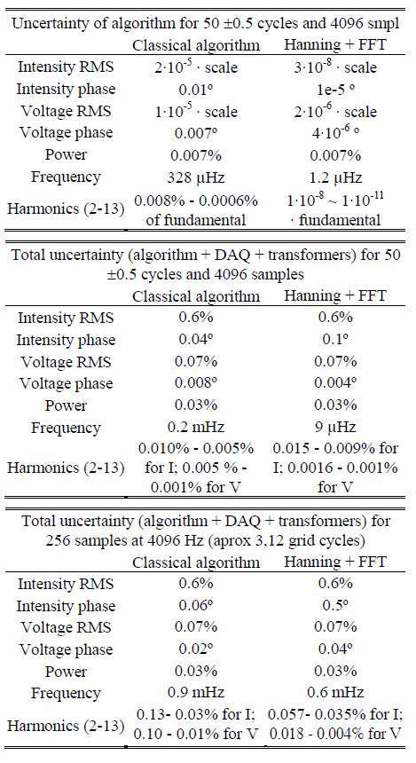
According to the ISO guide, GUM [27], each input deviation is modelled by a rectangular probability distribution. The sources of uncertainty of this system have been divided in four classes and their value have been estimated from data of DAQ and transformers specification (type B evaluation) [28]. For operation within ± 1ºC of the DAQ self-calibration temperature and gain equal to 1, we obtain the following values.
I. Offset and its temperature drift: completely correlated input quantities (constant, in absolute value, in each synthesized sample). uI = 864 μV at DAQ output.
II. Gain error, its temperature drift and stability: completely correlated input quantities (constant in relative value, urel = u(x)/|x|, in each synthesized sample). uII = 0.14% for V; uII = 1% for I. This value is the root sum square of transformer ratio error, DAQ gain error, gain temperature coefficient and long term stability.
III. Quantization, noise, linearity, time jitter, settling time and cross talk: not correlated input quantities (simulated as uniform noise in synthesized sample). uIII = 0.004 V for voltage; uIII = 0.0046 V for current, at DAQ output. This value is the root sum square of transformer linearity error and DAQ quantization, noise and nonlinearity.
IV. Phase error due to sequential A/D conversion of the input channels (simulated as a interchannel delay due to sequential scanning). Phase error of transformers can also be added here to the simulation (it has been not introduced in the simulation due to lack of data from manufacturer, but this mainly affects to power measurement).

Two measuring algorithms have been compared. One is based on FFT as it is shipped with LabVIEW. Its frequency guess input is taken from last measure since frequency is slow varying in grid-connected systems. Other alternative is to compute values by direct application of RMS and Fourier definitions (stated below classical algorithm). RMS is computed as root square sum of values and harmonics are computed dot multiplying the signal by sine-cosine functions (neither windowing nor 2N number of samples are required).
The first step in classical algorithm is estimate frequency from zero crossing of voltage to neutral, averaged on tree phases. To avoid wrong detections, a butter worth band-pass filter was applied forward and backwards and extremes of the signal were removed. In addition, an adjusted 5-point line gave the estimate of zero crossing and finally zero crossing is accepted if estimate is around the centre of the interval. This algorithm was validated in open field. Based in the estimated frequency, RMS values were easily computed based in an integer number of cycles (starting at 45º of the signal for best sensitivity). Phases were calculated based in time lag between zero crossing. Harmonics were computed dot multiplying the original signal with a sine and a cosine function of the corresponding multiple order of grid frequency. This allows to avoid FFT burden of obtain 2N number of samples and it was quicker in previous versions of LabVIEW. It is possible to use a table of pre-calculated sine and cosine to speed up (frequency is the same in all phases and for V and I and it has a narrow margin of variation) but this would increase uncertainty in long samples.
In LabVIEW versions prior to 6.0, classical algorithm was quicker than FFT. In contrast, Hanning +FFT algorithm run now approximately at same speed than classical. Classical version is quicker when less than 20 harmonics or no harmonics are computed, but it slows down with increasing number of harmonics calculated, in contrast with FFT. Hanning FFT is generally more precise than classical, but it is more sensitive to noise (when a real signal is applied, uncertainties are similar). DFT algorithm is about 50 % slower and simulation has shown that its uncertainty is similar to Hanning +FFT.
Table 1: Uncertainty estimation from simulation
V. ANALYSIS OF DATA
The fundamental variables of wind turbines have been related to generator speed, pitch, electrical power and wind speed and the information given by the manufacturer has been checked. As a sample, some figures will be shown next.
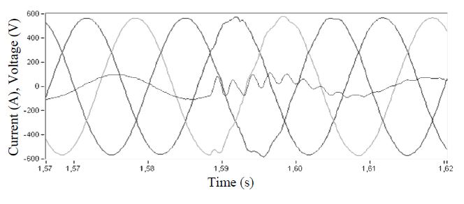
Voltage and current distortion can be easily viewed in low voltage at WT starting or stopping [29]. Connection of a capacitor bank is shown in Fig. 5, where waveforms of 563 V (690√2/√3) of amplitude are tree phase to neutral voltage waveforms. Current of R phase the smaller waveform experience ninth harmonic resonance for one grid cycle (similar behaviour is found in rest of phases).
Nevertheless, the effect of switching operations in WT are notably decreased at PCC due to higher short-circuit power, use of electronics and non simultaneous connection o disconnection [30]. Measurements have shown that simultaneous switching of more than three WT are unlikely to happen in this farm of 18 WT and complex orography.
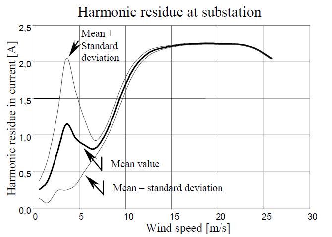
Distortion levels are bigger in DFIG due to the rotor converter, which commutes at 8 kHz. High order harmonics and interharmonics appear when the rotor converter is operating. High frequency harmonics are largely filtered by WT and substation transformers. Currents in neutral conductor are responsible of a 3rd harmonic in phase-to-neutral voltage. Nevertheless, this harmonic is blocked due to Dy11 connection of the transformer. Current harmonics are lower than voltage ones, even in DFIG, due to the high inductance of filter choke and transformer. Current harmonics are only important during switching operation, especially during starting and stopping events that occurs mainly around 4 or 5 m/s wind speeds. Fig. 6 displays current harmonic residue versus wind speed (thin lines represent the limit containing 62 % of measures). Harmonic residue has been used instead of THD – total harmonic distortion since, during switching operations, RMS value of distortion is comparable to fundamental component.
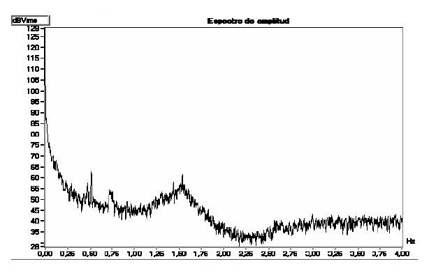
Power at WT shows fluctuations in power corresponding to blade passing the tower approximately 1,54 Hz and its submultiples half (0,75 Hz) and whole (0,5 Hz) revolution– (similar results have been found in Borja substation and in the WT). Fig. 7 shows the averaged spectrum of the generated power at Remolinos substation [31, 32, 33]. Nevertheless, mean fluctuation is small compared to the nominal power of the farm due to partial cancellation of oscillation. The mean values (average of module) of oscillation showed in Fig. 7 for a wind farm of 11,2 MW at 8-10 m/s are 1122 W at 1,54 Hz, 500 W at 0,74 Hz and 1400 W at 0,5 Hz.
In a time-frequency SFFT analysis of a WT shown in Fig. 8 we could see that maximum fluctuations occur at connexion of WT and in second place, at connexion of a capacitor bank. Good results are achieved using Hanning window (256 samples minimum) and overlapping (50 % minimum). Winger-Ville distribution and S-Transform have been tested and discarded for this application due to the presence of a wide spread of components [34, 35].

VI. CONCLUSIONS
A new portable measuring system has been designed to meet the requirements for PQ analysis of wind energy. It makes possible to record hours of non-stopping waveforms at a high sampling rate or, alternatively, to operate as a data logger.
The uncertainty of a measuring algorithm based in FFT and other based in direct application of RMS and harmonic definitions have been compared through Monte-Carlo simulation. Data from simulation show that the main source of uncertainty is the transformers and uncertainty from algorithm is negligible.
REFERENCES
[1] Hansen, K.S., Larsen, G. (1999) “Cut-in Note: Database on wind characteristics”, Wind Engineering, 23(3), 177-181. Available: http://www.winddata.com/
[2] J.R. Ubeda, M.A.R. Rodríguez García, “Reliability and production assessment of wind energy production connected to the electric network supply” IEE Proc.-Gener. Transm. distrib.. Vol. 146, Nº 2, March 1999, pp 169-175.
[3] R. Criado, J. Soto, J.M. Rodríguez, et al. “Analysis and control strategies of wind energy in the Spanish power system” International Conference on Large High Voltage Electric Systems, CIGRÉ. 2000.
[4] C.L. Masters, J. Mutale, G. Strbac, S. Curcic and N. Jenkins, “Statistical evaluation of voltages in distribution systems with embedded wind generation”. IEE Proc.-Gener. Transm. Distrib. Vol. 147, Nº 4, July 2000, pp. 207-212.
[5] T. S. Nielsen, A. Joensen, H. Madsen, L. Landberg, G. Giebel. “A New Reference for Wind Power Forecasting”, Wind Energy, 1, 25-45. September 1998.
[6] Wind Turbine Generator Systems–Part 21: Measurement and assessment of power quality characteristics of grid connected wind turbines, IEC61400-21.
[7] Guide for recorder and data acquisition requirements for characterization of power quality events, IEEE Standard P1159.1, draft. Available: http://grouper.ieee.org/groups/ 1159/1/keypts.html.
[8] Electromagnetic Compatibility (EMC)–Part 4: Testing and measurement techniques. Power quality measurement methods 61000-4-30, Draft version.
[9] A. Cuerva. “Some aspects on wind turbines monitoring. General considerations and loads on horizontal wind turbines”. Informes Técnicos Ciemat. 1996.
[10] J. Balcells, F. Daura, R. Esparza, R. Pallás. “Interferencias Electromagnéticas en Sistemas Electrónicos”. Marcombo. 1991.
[11] Electromagnetic Compatibility (EMC)–Part 3: Limits–Section 3: Limitation of Voltage Fluctuations and Flicker in Low- Voltage Supply Systems, IEC-EN 61000-3-3, 1994.
[12] S. Caldara, S. Nuccio, C. Spataro. “A Virtual Instrument for Measurement of Flicker”, IEEE Trans. Instr. Meas., Vol. 47, pp. 1155-1158. October 1998.
[13] Instrument transformers – Part 2 : Inductive voltage transformers, IEC 60044-2 Ed. 1.1 Consolidated Edition, Nov 2000.
[14] Instrument transformers – Part 1: Current transformers IEC 60044-1, Dec1996.
[15] A. Albers, H. Klug, D. Westermann, “Cup Anemometry in Wind Engineering, Struggle for Improvement”, DEWI Magazin Nr. 18, Feb 2001. http://www.dewi.de/dewi/magazin/ 18/04.pdf
[16] A. Albers, H. Klug, D. Westermann, “Outdoor Comparison of Cup Anemometers”, DEWI Magazin Nr. 17, August 2000, available at http://www.dewi.de/ dewi/magazin/17/02.pdf
[17] Ammonit, “Wind Measurement for accurate energy predictions”. Available: http://www.ammonit.de/knowhow.html
[18] International Energy Agency: Expert Group Study on Recommended Practices for Wind Turbine Testing and Evaluation, Wind Speed Measurement and Use of Cup Anemometry, 1999.
[19] H. Mellinghoff, A. Albers, H. Klug, “SODAR Measurements in Complex Terrain”, DEWI Magazin Nr. 17, August 2000. Available: http://www.dewi.de/ dewi/magazin/17/03.pdf
[20] D. A. Spera, “Wind Turbine technology”. ASME Press, 1994. Chapter 8: Characteristics of the Wind.
[21] F. Santjer, G. J. Gerdes, R. Klosse. “Power Quality Measurements at Wind Turbines”. Power Quality, June 1997 proceedings, pp 283-292
[22] G. McNerney, R. Richardson, “The statistical smoothing of power delivered to utilities by multiple wind turbines,” IEEE Transactions on Energy Conversion, Vol. 7, No. 4, pp. 644- 647, Dec. 1992.
[23] Wind turbine generator systems – Part 12: Wind turbine power performance testing., IEC 61400-12, Feb 1998.
[24] A. V. Oppenheim, R. W. Schafer. “Discrete-time signal processing”. Ed. Prentice-Hall, 1989.
[25] “DAQCard™-700 User Manual”. National Instruments. 1996.
[26] Electromagnetic Compatibility (EMC)–Part 4, Section 7: General guide on harmonics and interharmonics measurements and instrumentation, for power supply system and equipment connected thereto, IEC-EN 61000-4-7, Aug 2002.
[27] ISO – Guide to the expression of uncertainty in measurement, 1995.
[28] S. Caldara, S. Nuccio, C. Spataro. “Measurement Uncertainty Estimation of a Virtual Instrument”, IMTC 2000. Proceedings of the 17th IEEE, pp 1506 -1511 vol.3.
[29] Torbjörn Thiringer. “Power Quality Measurements Performed on a Low-Voltage Grid Equipped with Two Wind Turbines”. IEEE Trans. on En. Conv.. Vol. 11, No. 3, pp. 601-606. 1996.
[30] Heier, Siegfried. “Grid integration of wind energy conversion systems”. John Wiley & Sons Ltd.
[31] N. Visbøll, A. L. Pinegin, T. Fischer, J. Bugge. “Analysis of Advantages of the Double Supply Machine With Variable Rotation Speed Application in Wind Energy Converters”. DEWI Magazin Nr. 11, August 1997. Available: http://www.dewi.de/ dewi/magazin/11/08.pdf
[32] A. Feijoo, J. Cidras. “Analysis of mechanical power fluctuations in asynchronous WECS”. IEEE Transactions on Energy Conversion, Vol. 14, No. 3, pp. 284-291. Sept. 1999.
[33] E. Bossanyi, Z. Saad-Saoud and N. Jenkins. Prediction of Flicker Produced by Wind Turbines. Wind Energy 1, pp 35-51. 1998.
[34] Igor Djurovic, Ljubisa Stankovic. “A Virtual Instrument for Time-Frequency Analysis” IEEE Trans. on Instr. Meas. Vol. 48, No. 6, pp. 1086-1092. 1999.
[35] Tomasz P. Zielinski. “Joint Time-Frequency Resolution of Signal Analysis Using Gabor Transform” IEEE Trans. on Instr. Meas. Vol. 50, No. 5, pp. 1436-1444. 2001.
Manuscript received May 5, 2000. This work was supported in part by Department of Education and Culture of Aragón (B134/98 grant) and by Compañía Eólica Aragonesa S.A. (CEASA).
The authors are with CIRCE Foundation and the Electrical Department of Electrical Engineering, Zaragoza University, Spain (e-mail: joako@posta.unizar.es; msanz@posta.unizar.es, llombart@posta.unizar.es, aabayod@posta.unizar.es).
