Published by 1. Dominik DUDA, 2. Krzysztof MAŹNIEWSKI, 3. Bernard WITEK, Silesian University of Technology, Faculty of Electrical Engineering, Department of Power System and Control
ORCID: 1. 0000-0003-3247-2814; 2. 0000-0003-4357-6432, 3. 0000-0001-6732-9298
Abstract. Selected problems occurring in distance protection systems during earth faults in high voltage overhead cable lines (HV) were analyzed. The Alternative Transients Program (ATP) environment was used to simulate and model the phenomena. The influence of such factors as: fault location, arrangement of HV cables in the excavation, configuration of the return conductors and the earthing resistance of the return conductors was analyzed. The obtained results make it possible to verify the criteria for detecting earth faults in HV networks.
Streszczenie. Przeanalizowano wybrane problemy występujące w układach zabezpieczeń odległościowych podczas zwarć doziemnych w liniach napowietrzno-kablowych wysokiego napięcia (WN). Do symulacji i modelowania zjawisk wykorzystano środowisko Alternative Transients Program (ATP). Zbadano przebiegi prądów i napięć fazowych, składowe symetryczne prądu oraz położenie fazorów impedancji doziemionej fazy. Przeanalizowano wpływ takich czynników jak: lokalizacja zwarcia, ułożenie kabli WN w wykopie, konfiguracja żył powrotnych oraz rezystancja uziemienia żył powrotnych. Uzyskane wyniki pozwalają na weryfikację kryteriów wykrywania zwarć doziemnych sieci WN. (Działanie zabezpieczeń odległościowych podczas zwarć doziemnych w sieciach wysokich napięć ze wstawkami kablowymi).
Słowa kluczowe: sieci WN; zwarcia doziemne; modelowanie i symulacja zwarć; zabezpieczenia napowietrzno-kablowych linii elektroenergetycznych; kryterium impedancyjne.
Keywords: HV networks; Phase-to-earth faults; Faults modeling and simulation; Overhead-cable power lines protection; Impedance criterion.
Introduction
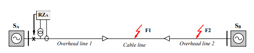
When considering the fault protection of HV networks, the cable line is often omitted or treated as a homogeneous element of the overhead line. However, such an approach may result in the incorrect operation of fault (especially earth-fault) protection, and lead to thermal damage due to the flow of large currents of significant value [1,2,10]. The purpose of this paper is to present, how the factors like: configuration of cable routing and the way of connecting and earthing the return cores affect the correct earth-fault detection by the protection of the HV overhead line with a cable insert. The assumed simulation model has been described and verified in the previous authors paper [15].
The main aspects of this article (the fault transients from the point of view of the HV lines distance protection) is relatively poorly described in the literature. Therefore chapter 2 concentrates on selected simulation results of the earth-faults. Voltages and currents waveforms as well as impedance trajectories illustrate the estimated impedance changes during the fault transient state i.e. include the fault inception and the final locus of the impedance phasor.
The simulation results can be particularly useful for determination of critical power system protection values, that are used for fault detection in the protected overhead cable line [9].
The impact of selected factors on the earth fault protection criteria
Two basic criteria can be applied to protect the HV line against the effects of earth faults: an analysis of the position of the impedance phasor within the complex plane, and detection of the zero-sequence current and voltage. The first criterion is used, for example, in distance protection. The second criterion is used for directional earth-fault protection [14].
As described in [15] HV cable lines differ in the configuration of the return conductors and the positioning of the cables within the trench. Moreover, aging factors affect the earthing resistance of the return conductors. In the following section, we use the ATP_Draw model of the overhead-cable network (Fig. 1) to analyze the impact of these factors on the selected distance protection criteria. This chapter describes in detail the simulations results for the CB system as the most complex one [3,4].
Full simulation tests were also carried out for the BE and SPB systems, adopting the same input data and changing only the way of connection and grounding of the return conductors [5,6].
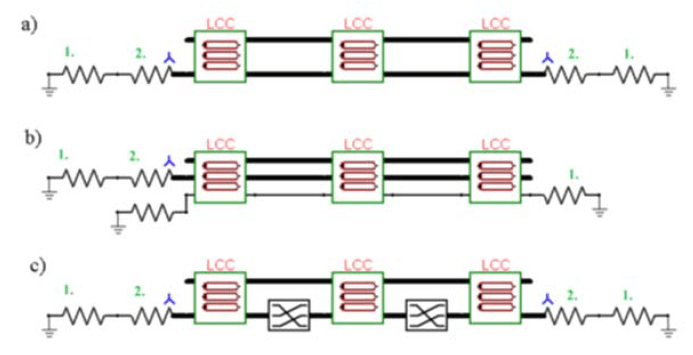
BE, CB, and SPB variants of the cable line were modelled in ATP environment [11,12]. The configuration of the return conductors differed between each variant (Fig. 2).
Influence of the cable line return conductors earthing configuration
For this scenario, we make the following assumptions:
• the cables were deployed in a flat formation,
• the return conductors had an earthing resistance of RG = 5 Ω,
• the phase L3 fault occurred at t = 0.1 s midway along the cable line, and
• the fault resistance was RF = 5 Ω.
The simulations ran for a total of 0.25 s. Table 1 summarizes the results, showing RMS and maximum values of the phase voltages and currents in the return conductors, in addition to individual symmetrical current components, for the BE, CB, and SPB systems. Table 2 presents the parameters that define the final locus of the phase-to-ground impedance phasor within the complex plane, i.e. during short-circuit steady-state.
Fig. 3 shows an example of the phase voltage and current waveforms measured at the protection point (indicated by RZA in Fig. 1). Among the considered configurations, the BE system featured the highest peak value of the phase L3 current. The lowest peak value of the phase L3 current occurred in the SPB system. The BE system also featured the most significant decrease in L3 phase RMS voltage Uc. In contrast, the SPB system featured the smallest such reduction. The smallest values of zero- and negative-sequence currents also occurred in the SPB system.
Table 1. RMS and maximum values of the phase voltages and currents, in addition to individual symmetrical current components for the BE, CB, and SPB systems.
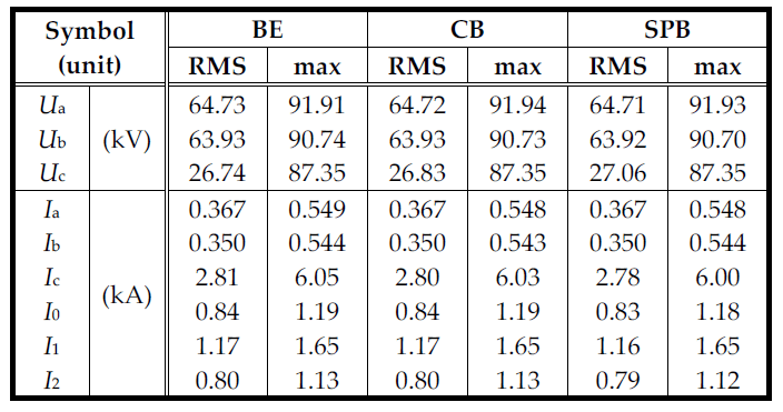
Table 2. Fault steady-state (final) values of resistance (Ω), reactance (Ω), and earth-fault impedance modulus (Ω) (phase L3), for the BE, CB, and SPB systems.
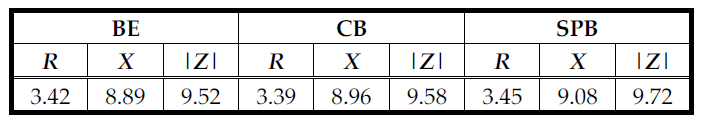
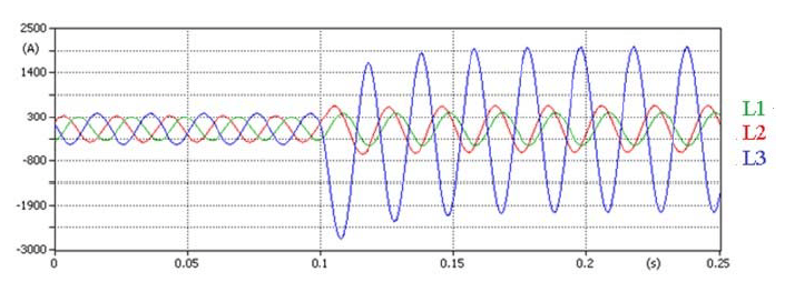
Fig. 4 shows the phasor trajectories of the short-circuit impedance for the BE, CB, and SPB systems. Among other factors, the trajectories are defined by the measurement window used to estimate the orthogonal components, and by the occurrence of the non-periodic current component. The graphical representation of the impedance trajectories required ATP output files conversion and development with use of the fault recording program iRec [7,8].
The simulation results presented in Table 2 and Fig. 4 show that the return conductor configuration has a modest influence on the trajectory and final locus of the impedance phasor.
Influence of the cable formation
The short-circuit impedance is also dependent upon the formation of phase cables within the cable line. Simulations were carried out for both the flat and trefoil cable formations. The simulations used the same return conductor earth resistance (5 Ω) and transition resistance (5 Ω) as the previous simulations. For these simulations we only considered use of the CB system. Fig. 5 depicts the flat and trefoil cable formations.
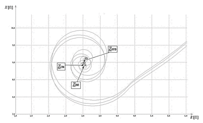
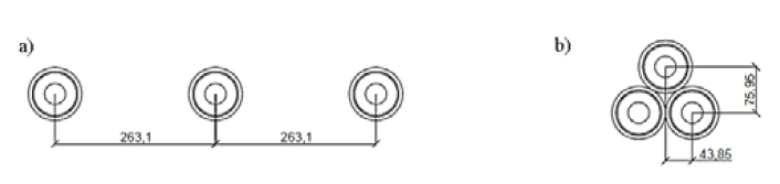
Table 3 presents the parameters that define the final locus of the phase-to-ground impedance phasor within the complex plane, during steady-state short-circuit operation. The difference column shows the difference in parameter values between the two cable formations.
Table 3. Final values of resistance (Ω), reactance (Ω), and earth fault impedance modulus (Ω) (phase L3), for the flat and trefoil cable formations, when using the CB system.
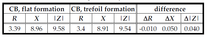
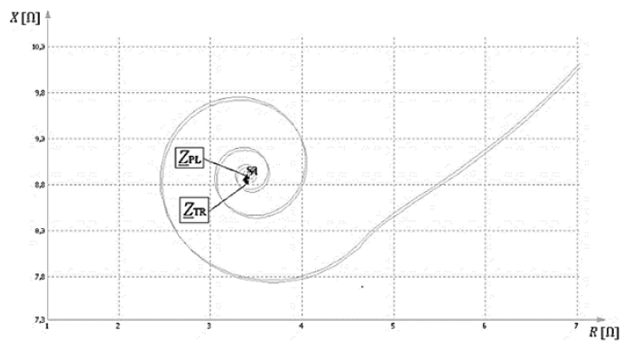
Fig. 6 shows the phasor trajectories of the short-circuit impedance for the flat and trefoil cable formations. The results show that the cable formation has a modest impact on the trajectory and final locus of the impedance phasor.
Influence of return conductor earthing resistance
In real applications, HV cable return conductors are typically earthed at a minimum of one location. Among other benefits, such earthing distributes the electric field radially inside the cable insulation. Moreover, due to aging phenomena such as corrosion, the earthing resistance (RG) of the cable return conductors increases over time. Therefore, we simulated two different values of the return conductor earthing resistance: 5 Ω and 10 Ω. Both simulations used the CB system. As for all previous simulations, we used a transition resistance at the fault location of 5 Ω. Table 4 presents the parameters that define the position of the phase-to-ground impedance phasor within the complex plane, during steady-state short-circuit operation. The difference column shows the difference in parameter values between the earthing resistances of 5 Ω and 10 Ω.
Table 4. Steady-state values of resistance (Ω), reactance (Ω), and earth-fault impedance modulus (Ω) (phase L3), for different values of return conductor earthing resistance, when using the CB system.

During the simulations, the two different earthing resistances resulted in noticeably different peak values of the return conductor currents. As expected, the currents were larger for RG = 5 Ω than for RG = 10 Ω.
Fig. 7 shows the phasor trajectories of the short-circuit impedance for both values of earthing resistance. Both the trajectories and final locus for each impedance phasor differ for the two earthing resistances. From these results, we determine that the earthing resistance of the HV cable return conductors can significantly impact the characteristic earth-fault values – particularly the resistance component of the impedance phasor. 2.4. Fault location influence For the simulations in this section, the parameters were configured as follows:
• the cables were deployed in a flat formation,
• return conductors had an earthing resistance RG = 5 Ω,
• the fault occurred at t = 0.1 s, and
• the fault resistance was RF = 5 Ω.

Each simulation ran for 0.25 s, using the CB system. Two different fault locations were considered, as shown in Fig 1. The fault at F1 was located within the cable line, and the fault at F2 was located within the overhead line. Table 5 summarizes the simulation results, showing RMS and maximum values of phase voltages and currents, in addition to individual symmetrical current components for each fault location. The parameters provided in Table 6 define the final locus of the phase-to-ground impedance phasor. The difference column shows the difference in parameter values between the two different faults.
Fig. 8 shows the current waveforms in the return conductors. The waveforms differ significantly from one another. The current flowing through the cable return conductors during the short-circuit at F1 is both larger and more asymmetric, in terms of the current waveforms in individual conductors, than during the short-circuit at F2.
Table 5. RMS and maximum values of the phase voltages and currents, in addition to symmetrical current components for faults at F1 and F2 (Fig. 1), when using the CB system.

Table 6. Steady-state values of resistance (Ω), reactance (Ω), and earth-fault impedance modulus (Ω) (phase L3) for faults at F1 and F2, when using the CB system.
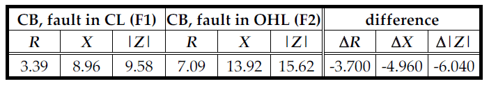
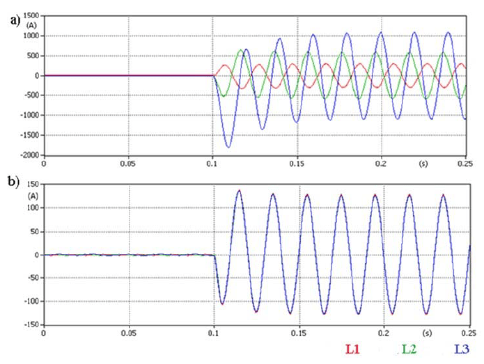
Fig. 9 shows the voltage waveforms measured at the transposition point of the return conductors. For both fault locations, a sharp increase in voltage occurs between the return conductors and the ground at the instant the fault arises. Moreover, the peak voltage across the return conductors is much higher during the cable line (F1) fault.
Fig. 10 shows the phasor trajectories of the L3 phase impedance for both fault locations. A noticeable difference can be observed between both the trajectories and the final locus of the phasors for the two different fault locations.


Summary of the simulations
Fig. 11 summarizes the simulation results for each of the three considered cable systems. The figure shows the peak short-circuit currents and individual symmetrical current components, in addition to the defining parameters of the short-circuit impedance phasor. The results show that the configuration of the return conductors has a relatively small impact on the selected short-circuit parameters, and hence should not affect the correctness of the earth-fault detection.
Fig. 12 compares use of the flat and trefoil cable formations, showing the differences in peak short-circuit current and individual symmetrical current components, in addition to the defining parameters of the short-circuit impedance phasor.
The simulation results show that the cable formation substantially impacts the phase values during a short-circuit within the considered cable line. For the CB and SPB systems, use of the trefoil formation results in a larger short-circuit current, a higher zero-sequence current, and a noticeable decrease in short-circuit impedance. Among each of the considered systems, the cable formation has the greatest impact on the considered short-circuit parameters in the SPB system.
The simulation results show that the earthing resistance of the return conductors impacts the phase values during a short-circuit within the considered cable line. The increase in earthing resistance causes the peak values of all measured quantities to decrease. Moreover, an increase in grounding resistance causes an increase in the real component of the L3 phase impedance, altering the final position of the L3 phase impedance phasor. Among each of the considered systems, variations in earthing resistance most strongly affect the BE system, and least strongly affect the SPB system.

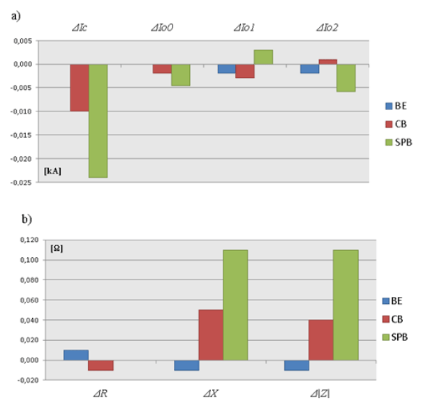
Fig. 13 compares two different grounding resistances: RG = 5 Ω and RG = 10 Ω. The figure shows the differences in peak short-circuit currents and individual symmetrical current components, in addition to the defining parameters of the short-circuit impedance phasor.
Simulations were also conducted to determine the impact of the fault location on the selected fault parameters. The fault locations F1 and F2 are indicated in Fig. 1.
Fig. 14 summarizes the simulation results, showing the differences in short-circuit current and the peak values of individual symmetrical current components, in addition to the defining parameters of the short-circuit impedance phasor.


The impact of fault location on the correctness of the short-circuit loop impedance measurement is the smallest for the SPB system. The impact is largest for the BE system.
Conclusion
The article describes selected problems associated with the operation of HV over-head-cable lines. A particular focus was placed upon the earth-faults detection with use of the impedance (distance) criterion.
Further research may include a comprehensive analysis of the influence of the considered factors on the correctness of a short-circuit detection in such lines. More extensive research could determine the optimal operation of such lines, both in normal conditions and in fault conditions. Such a knowledge would engender the correct detection of short-circuits – particularly earth faults.
REFERENCES
[1] Anders G.J., Rating of Electric Power Cables in Unfavorable Thermal Environment; John Wiley and Sons: Hoboken, NJ, USA, 2005.
[2] Duda D., Szadkowski M., Żmuda K., Current problems of 110 kV cable lines (mainly municipal) designing and operating; Wiadomości Elektrotechniczne, 2014, 4, 22-26. (In Polish)
[3] CIGRE TB 531: Cable Systems Electrical Characteristics; WG B1.30, April 2013.
[4] CIGRE TB 283: Special Bonding of High Voltage Power Cables; WG B1.18, October 2005.
[5] CIGRE TB 797: Sheath Bonding Systems of AC Transmission Cables – Design, Testing, and Maintenance; WG.B1.50, March 2020.
[6] IEEE Guide for Bonding Shields and Sheaths of Single-conductor Power Cables Rated 5 kV through 500 kV; IEEE Standard Association: Piscataway, NJ, USA, 2014. http://dx.doi.org/10.17531/ein.2020.1.3.
[7] https://zaz-en.pl/pl/produkty/izaz-tools – Protective devices testing software. (In Polish)
[8] Krasinski J., Selected Aspects of High Voltage Cable Line Parameters and Configuration Influence on Earth Fault Waveforms; Master Thesis. Silesian University of Gliwice, 2020. (In Polish)
[9] Witek B., Modeling of the Earth Faults in overhead – Cable HV Lines; Energetyka nr 2/2016, s. 99-104. (In Polish)
[10] Witek B., Some Aspects of Power System Protection in Cable and Overhead-Cable HV Lines; Energetyka nr 5/2016, s. 281-285. (In Polish)
[11] Rosołowski E., Computer Methods of Electromagnetic Transients Analysis. Oficyna Wydawnicza Politechniki Wrocławskiej, Wrocław 2009. (In Polish)
[12] Arrillaga J., Watson N.R., Computer Modeling of Electrical Power Systems; Wiley & Sons, Chichester 2001.
[13] Witek B., Selected issues of electrical power system computation and design. Vol. 1, Power transmission system; Gliwice, Wydawnictwo Politechniki Śląskiej, 2019.
[14] Ungrad H., Winkler W., Wiszniewski A., Protection Techniques in Electrical Energy Systems; Marcel Dekker, New York 1995.
[15] Duda D., Mazniewski K., Witek B.: Cable Inserts Modeling in Steady State Operating Conditions of High Voltage Networks. Przegląd Elektrotechniczny 2022, (to be published).
Authors: Department of Power System and Control, Faculty of Electrical Engineering, Silesian University of Technology, 44-100 Gliwice, Poland; Dominik Duda PhD (EE), e-mail: dominik.duda@polsl.pl; Krzysztof Maźniewski PhD (EE), e-mail: krzysztof.mazniewski@polsl.pl; Bernard Witek PhD (EE), e-mail: bernard.witek@polsl.pl;
Source & Publisher Item Identifier: PRZEGLĄD ELEKTROTECHNICZNY, ISSN 0033-2097, R. 99 NR 6/2023. doi:10.15199/48.2023.06.19
