Published by 1. Yuly Bay, 2. Nikolay Ruban, 3. Mikhail Andreev, 4. Alexandr Gusev, Tomsk Polytechnic University. ORCID. 1. 0000-0001-9928-408X, 2. 0000-0003-1396-9104, 3. 0000-0002-6420-4374, 4. 0000-0003-0814-2356
Abstract. The penetration of renewable energy sources (RES) into the electricity supply is gaining popularity all over the world, including countries that have large oil and gas reserves, since only the development of alternative energy will help avoid regression and take a green path development, reducing the damage to the environment. According to estimates of the International Energy Agency (IEA), the capacity of RES units built in China in 2016 was 34 GW, and Australia is one of the world leaders in the photovoltaic power plants installation, the share of which in the Australian electricity production exceeds 3%. It should be noted, that the final power generation capacity and stability are stochastic (probabilistic) in nature. Unlike the classical type generator, the output RES characteristics depend on the geographical features of the installation area, the season, and prevailing winds. Risks associated with inaccurate knowledge of the cumulative distribution function (CDF) describing these sources, as well as environmental uncertainties, are the reasons why it is more difficult for distribution network operators (DNO) to take RES into account in the power balance calculations. The wind speed CDF clarification can provide significant assistance in predicting the RES power production.
Streszczenie. Według szacunków Międzynarodowej Agencji Energetycznej (IEA) moc jednostek OZE wybudowanych w Chinach w 2016 roku wyniosła 34 GW, a Australia jest jednym ze światowych liderów w instalacji elektrowni fotowoltaicznych, której udział w australijskiej produkcji energii elektrycznej przekracza 3%. Należy zauważyć, że końcowa moc i stabilność wytwarzania energii ma charakter stochastyczny (probabilistyczny). W przeciwieństwie do generatora typu klasycznego, charakterystyka wyjściowa OZE zależy od cech geograficznych obszaru instalacji, pory roku i dominujących wiatrów. Ryzyko związane z niedokładną znajomością skumulowanej funkcji dystrybucji (CDF) opisującej te źródła, a także niepewności środowiskowe powodują, że operatorom sieci dystrybucyjnych (DNO) trudniej jest uwzględnić OZE w obliczeniach bilansu mocy. Wyjaśnienie prędkości wiatru CDF może zapewnić znaczącą pomoc w przewidywaniu produkcji energii z OZE. (Analiza statystyczna rozkładów probabilistycznych prędkości wiatru do oceny energetyki wiatrowej w różnych regionach)
Keywords: power system, wind speed time series, probability density function, cumulative distribution function.
Słowa kluczowe: energetyka wiatrowa, rozkład statystyczny.
Introduction
The structure and principles of power system management are becoming more and more complicated. Over the past 15 years due to the insufficient capacity of traditional generation sources, in most developed countries, for reasons of ensuring energy, environmental safety, etc., preference is given to RES, which is being actively introduced in China, Europe and the United States, and the total generated capacity is approximately 2195 GW. Due to this, the total RES capacity is expanding, which leads to an increase in power system stochastic processes.
In the classical cases, the electrical power system (EPS) is a «vertically» arranged system, where a number of operating factors and controlled variables are clearly defined and set within a specific way, established by the DNO [1]. However, in cases of renewable generation penetration, especially in large amount, there is a problem of discrepancy between the generated capacity and the electricity demand. Poor predictability associated with the current wind flow strength, which does not coincide in time with the required capacity, leads to mode dispatching problems. The RES, unlike traditional generators, restructuring EPS into a «vertical-horizontal» one [2], adding uncertainties in management that require further research and forecasting.
The ability and accuracy of forecasting is limited by the statistical information quality or methods of its processing. For example, in these works [3], deterministic methods were used to predict power generation, in order to represent RES as classical. In the articles [4], the probability distribution functions were selected for the input and output characteristics by the statistical analysis methods and testing by goodness of fit criteria. There are also studies devoted to the investigation of the power system units probabilistic characteristics, such as the expected value and standard deviation, the calculation of which contributes to the calculation of the optimal RES implementation capacity in order not to loss of steady state and transient stability.
The wind speed probability distribution approximation
The distribution law choice depends on many factors, including the specifics of the problem. To determine the estimated wind speeds of low frequency (dependence on the wind rose chart [5]), the maximum wind speeds possible in a particular area [6]), the main requirement is a reliable coincidence of empirical and theoretical distributions in the high-value range. The approximation itself as applied to the wind speed distribution was initially widely used for statistical extrapolation of the maximum wind speeds [7]. Subsequently, the approximation of the wind speed distribution by the Weibull and Weibull-Goodrich laws has become one of the most widely used [8]. Along with this law, the normal distribution law is often used, but a large sample size is required to reliably estimate the distribution parameters.
There are papers [9] that claim that the probability distribution is also well described by the lognormal distribution. The laws that can be used for modelling the wind speed, as well as their parameters, are given in the Table 1.
Table 1. Expressions of statistical distributions

where k – shape parameter, c – scale parameter, Г – gamma function, α,β,η – parameters of distributions, – normal distribution
The form of the distribution law also depends on the set of observations. In such situations, the distributions of the criteria statistics are often unknown, which is a frequent source of incorrect conclusions.
For optimal research, it is necessary to use several methods to determine the possible distribution law, even before using the goodness of fit criteria. Several well-known methods have been used to determine the various distributions parameters, out of which the method of moments, the graphical method, and the maximum likelihood method. In the case of using the graphical method, it has the advantage of simplicity, however, the accuracy of the input parameters estimating can be insufficient [10]. The likelihood method, on the contrary, has good accuracy, but to achieve it, it is required to use iterative methods [11]. The method of moments equates a certain number of statistical moments of the sample with the corresponding population moments [12]. The use of these methods (at least the maximum likelihood method and method of moments) usually implies that there is an assumption of the possible probability laws that are available in the wind time series. However, in the case of considering the unexplored wind time series, it is more logical to use the graphical or brute force method [13], with subsequent evaluation by several goodness of fit criteria.
The goodness of fit tests
The suitability of the chosen theoretical distribution for describing the empirical probability of a given meteorological argument is verified using the goodness of fit criteria. In this article, we will use Pearson’s chi-squared test [14] and Kolmogorov-Smirnov Goodness-of-Fit Test [15, 16], since the first of them is very sensitive to the dissimilarity of the values edges, the second allows us to more accurately assess the differences in the central regions.
Applying both criteria (with a given 5% significance level), the selected theoretical distribution function can be safely used for indirect calculations. For the measure of the difference between the theoretical and empirical distributions, Pearson takes the value X2 determined by the formula:
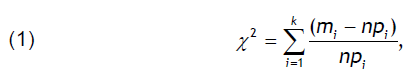
where n – the sample size, mi – the relative frequencies of the empirical distribution, pi – the corresponding theoretical probability densities, k – the gradations number.
Kolmogorov proposed another goodness of fit criteria, which, in contrast to the Pearson criterion, is based on a comparison of experimental and theoretical distributions integral laws.
As a measure of difference, A. N. Kolmogorov-Smirnov test uses the value:
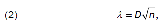
where n – the sample size, D – corresponds to the upper bound (the largest value of the difference between the considered and the original sample) |F*(xi) – F(xi)| = δ(xi).
Input wind time series data
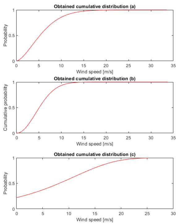
For the experiments, three samples of wind time series data with unknown CDF were taken. The sample size is between 9000 and 200000 volumes, depending on the example. The first sample (Fig. 1a) was taken from one of the graphical method experiments to study Weibul’s law parameters, and was randomly generated. The second time series is taken from the small-scale wind turbine power curve study (Fig. 1b) [17]. The third sample (Fig. 1c) is taken from the wind hourly NUTS 2 time series array [18].
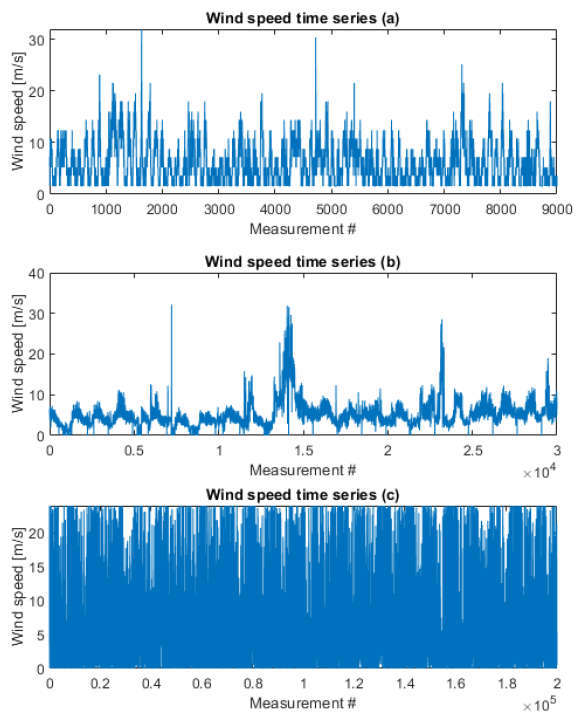
Based on the information provided, preliminary conclusions can be made about the wind values repeatability, maximum observed and average (mean) values. It should be noted, that in this case, all samples are not tied to particular months, but represent the full input data set for all the time [19]. The parameters that can be obtained before calculating the extracted CDF are shown in Table 2.
Table 2. Wind time series parameters

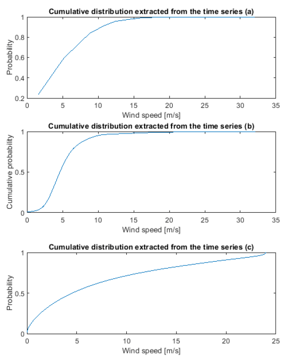
Before the process of finding a fitting CDF and checking it with the goodness of fit criteria, it is necessary to process the input wind data. To do this, we extract the unique values occurring in the wind time series, find the number of occurrences of each unique wind speed value, get the total number of measurements and get the cumulated frequency at the finish (Fig. 2).
A graphical analysis of wind speed CDFs
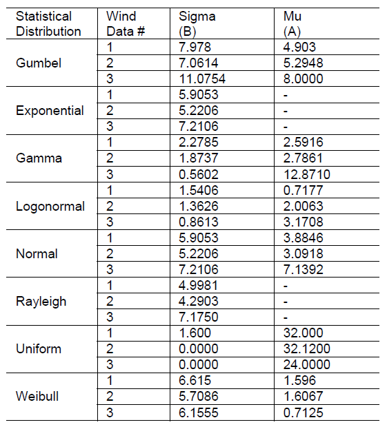
In order to determine the optimal PDLs, we need to estimate the shape and scale parameter of the curves. Using extracted wind data CDFs, we generate the corresponding PDs. According to the obtained PDs, using the graphical method in conjunction with additional ones, all parameters of possible PDLs are determined, to which the studied wind time series may belong. An example is shown in Fig. 3 for the first data array (a). All parameters of possible distributions are given in Table 3.

Fig. 3 shows eight PDFs, namely the Gumbel, Exponential, Gamma, Logonormal, Normal, Rayleigh, Uniform, and Weibull, fitted to the wind speed values. Graphically it can be observed that Logonormal PDF gives the best match. The Gamma, Rayleigh and Weibull distributions match the histogram to a lesser degree, and the remaining distributions provide the worst fits.
Similarly, these eight PDFs were also fitted to other two wind series data and it was observed that the Logonormal, Gamma, Weibull, and Rayleigh the best ones for further analyses.
The most widely used distribution of the selected laws is the Weibull distribution. It is easy to use and accurate for most wind conditions that may occur in research. The Rayleigh distribution is a simplified version of the Weibull distribution, characterized by its simplicity due to the use of only one parameter, which negatively affects the quality of the obtained characteristics, and it is not so often suitable. Gamma and lognormal distributions are also two-parameter, they are less common in wind descriptions, but they can be much better suited for a several wind time series [20] (depending on the wind samples specific values repeatability).
Table 3. Wind time series obtained distribution parameters
After that, the wind time series is checked using the Pearson’s chi-squared test and Kolmogorov-Smirnov Goodness-of-Fit test according to the laws selected above. For the first sample data, the Weibull distribution meets the goodness-of-fit criteria (Fig. 4a). The second one corresponds to the Rayleigh distribution (Fig. 4b).
For the third sample, the Gambel distribution and the normal distribution were the closest, but neither of them fully satisfied the Kolmogorov test. This may be due to the small number of distribution laws considered, which were proposed in the article, or to the complexity of the original law (multiparameter, multimodal distribution, etc.).
Thus, we can conclude that the tools for finding the probabilistic characteristics of the wind time series presented in this article are extensive, but not always sufficient for the most accurate description of complex laws. For some cases, it may be necessary to use more sophisticated and advanced methods to obtain reliable probabilistic parameters.
Conclusion
The study of the wind speeds CDF was based on real and accurate measurements of these values at three obviously different sites. The results showed that it was possible to fully determine the probabilistic characteristics corresponding to the goodness-of-fit criteria for two of them. Thus, for some investigated wind time series, it will be necessary to expand the initial list of possible CDFs.
The implemented capabilities for modeling the distribution from random variables allow us to model the CDF and PD for the RES active and reactive power of various configurations based on the specific territory wind models.
Acknowledgment – The work was supported by Ministry of Science and Higher Education of Russian Federation, according to the research project № МК-5320.2021.4.
REFERENCES
[1] Zhang, J., M. Cheng, and X. Cai. (2012). Short-Term Wind Speed Prediction Based on Grey System Theory Model in the Region of China. Przeglad Elektrotechniczny, 88 (7a), 67-71.
[2] Strzelczyk, F. (2009). Renewable energy sources in power system. Przeglad Elektrotechniczny, 85 (9), 340-349.
[3] Karaki, S.H., Chedid, R.B., Ramadan R. (1999). Probabilistic performance assessment of autonomous solar–wind energy conversion systems, IEEE Trans Energy Conversion, 14 (3), 766–772.
[4] Kruangpradit P., Tayati W. (1996). Hybrid renewable energy system development in Thailand, Renewable Energy, 8 (1–4), 514–517.
[5] Sohoni, V., Gupta, Sh., Nema, R. (2016). A comparative analysis of wind speed probability distributions for wind power assessment of four sites. Turkish Journal of Electrical Engineering & Computer Sciences, 24, 4724-4735.
[6] Giraldo, J., Castrillon, J., Granada-Echeverri, M. (2014). Stochastic AC Optimal Power Flow Considering the Probabilistic Behavior of the Wind, Loads and Line Parameters. Ingeniería e Investigación, 15, 529-538
[7] Soroudi, A., Aien M., Ehsan, M. (2012). A Probabilistic
Modeling of Photo Voltaic Modules and Wind Power Generation Impact on Distribution Networks. IEEE Systems Journal, 6 (2), 254-259.
[8] Malska, W. and D. Mazur. (2017). Analysis of the Impact of Wind Speed for Power Generation on the Example of Wind Farm. Przeglad Elektrotechniczny, 93 (4), 54-57.
[9] Akyuz, H., Gamgam, H. (2017). Statistical Analysis of Wind Speed Data with Weibull, Lognormal and Gamma Distributions. Cumhuriyet Science Journal, 38, 68-76.
[10] Ross, R. (1994). Graphical Methods for Plotting and Evaluating Weibull Distributed Data. Proceedings of the 4th Int. Conf. Properties and Applications of Dielectric Materials,1, 250 – 253.
[11] Cousineau, D., Brown, S., Heathcote, A. (2004). Fitting distributions using maximum likelihood: Methods and packages, Behavior Research Methods, Instruments, & Computers,36, 742–756.
[12] Prem, Ch., Siraj, A., Vilas, W. (2018). Study of different parameters estimation methods of Weibull distribution to determine wind power density using ground based Doppler SODAR instrument. Alexandria Engineering Journal, 57 (4), 2299-2311.
[13] Dongbum, K., Kyungnam, K., Jongchul H. (2018). Comparative Study of Different Methods for Estimating Weibull Parameters: A Case Study on Jeju Island, South Korea. Energies, 11 (2), 1-19.
[14] Seyit, A., Akdağ, A., D. (2009). A new method to estimate Weibull parameters for wind energy applications. Energy Conversion and Management, 50 (7), 1761-1766.
[15] Çelik, H., Yilmaz, V. (2008). A Statistical Approach to Estimate the Wind Speed Distribution: The Case of Gelibolu Region. Doğuş Üniversitesi Dergisi, 9 (1), 122-132.
[16] Bielecki, S. (2017). Reactive Power Demand – Verification of a Hypothesis of Normal Distribution Values). Przeglad Elektrotechniczny, 93 (9), 20-23.
[17] Loic, Q., Clement, J., Christian. E. (2014). Measuring the Power Curve of a Small-scale Wind Turbine: A Practical Example. Conference Proceedings Paper – Energies “Whither Energy Conversion? Present Trends, Current Problems and Realistic Future Solutions”, pp. 1-11.
[18] González-Aparicio, I., Monforti, F., Volker, P., Zucker, A., Careri, F., Huld, T., Badger, J. (2017). Simulating European Wind Power Generation Applying Statistical Downscaling to Reanalysis Data. Applied Energy, 199, 155-168.
[19] Rosas, P. A. C., Nielsen, A. H., Bindner, H. W., Sørensen, P. E., Lindahl, S. O. R., Nielsen, J. E. & Pedersen, J. K. (2004). Dynamic Influences of Wind Power on The Power System, Technical University of Denmark, Denmark, Forskningscenter Risoe.
[20] Lingfeng, W., Chanan, S., Andrew, K. (2010). Wind Power Systems: Applications of Computational Intelligence, Springer-Verlag Berlin Heidelberg.
Authors: Assistant of Division for Power and Electrical ngineering, Yuly Bay, Tomsk Polytechnic University, 30, Lenin Avenue, Tomsk, Russia, E-mail: nodius@tpu.ru; Associate professor of Division for Power and Electrical Engineering, Nikolay Ruban, Tomsk Polytechnic University, 30, Lenin Avenue, Tomsk, Russia, E-mail: rubanny@tpu.ru; Associate professor of Division for Power and Electrical Engineering, Mikhail Andreev, Tomsk Polytechnic University, 30, Lenin Avenue, Tomsk, Russia, E-mail: andreevmv@tpu.ru; Professor of Division for Power and Electrical Engineering, Aleksandr Gusev, Tomsk Polytechnic University, 30, Lenin Avenue, Tomsk, Russia, E-mail: gusev_as@tpu.ru.
Source & Publisher Item Identifier: PRZEGLĄD ELEKTROTECHNICZNY, ISSN 0033-2097, R. 97 NR 12/2021. doi:10.15199/48.2021.12.14
