Published by Mirosław WCIŚLIK, Paweł STRZĄBAŁA,
Kielce University of Technology, Department of Electric Engineering, Automatic Control and Computer Science
Abstract. The paper deals with an AC circuit containing the nonlinear load and a LC passive filter. Nonlinear load voltage at the power terminals proportional to the signum function of current is considered. The current-voltage characteristic of such load is unambiguous (without hysteresis). A quality analysis of the circuit voltages and currents was carried out. Distribution of active and reactive power for fundamental and higher harmonics in the circuit were also performed.
Streszczenie. W pracy analizowany jest obwód prądu przemiennego z przykładowym obciążeniem nieliniowym i filtrem biernym LC. Przyjęto obciążenie nieliniowe, którego napięcie na zaciskach zasilania jest proporcjonalne do funkcji signum prądu. Charakterystyka napięciowo – prądowa obciążenia jest jednoznaczna (bez histerezy). Przeprowadzono analizę jakościową przebiegów napięć i prądów obwodu. Wykonano analizy rozkładu mocy czynnej i biernej dla harmonicznej podstawowej i wyższych harmonicznych w obwodzie. Analiza oddziaływań w obwodzie systemu elektroenergetycznego z obciążeniem nieliniowym i filtrem biernym LC.
Keywords: nonlinear load, higher harmonics, reactive power compensation, interaction analysis.
Słowa kluczowe: obciążenie nieliniowe, wyższe harmoniczne, kompensacja mocy biernej, analiza oddziaływań.
Introduction
In order to improve energy efficiency and electricity savings, it is necessary to reduce the interaction between the power system and nonlinear receivers. For this purpose, LC passive filters are commonly used. These filters compensate the reactive power in the circuit and may reduce the flow of higher harmonics of current into the power system. Nonlinear loads, that most often disturb the quality of power supply voltage are arc furnaces and rectifiers [1]. In [2] it has been shown that nonlinear load with unambiguous current-voltage characteristics has a total reactive power equal to zero, and the reactive power of the first harmonic of this load is converted into the reactive power of the higher harmonics and fully transferred to the equivalent reactance of the supply circuit. This property is also characteristic for rectifiers. The phenomenon of power conversion in circuits with nonlinear loads and LC passive filters has not been analysed in the literature so far. Usually the nonlinear load is replaced by a simplified model of a current source. There is assumed that the nonlinear receiver is a generator of higher harmonics of current [3],[4],[5],[6]. In order to take into account the conversion phenomena, the AC circuit with LC passive filter and nonlinear load is considered. There was assumed that the voltage at terminals of nonlinear load is proportional to the current signum function. It is a model of the electric arc and a bridge rectifier.
Model of analyzed circuit
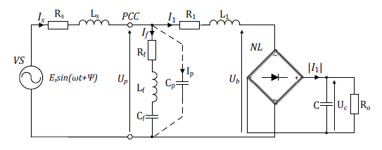
The analysed AC circuit is shown in Fig.1. The circuit contains bridge rectifier supplied by a sinusoidal voltage source with the amplitude Es and the angular frequency ω. The inductance Ls and resistance Rs represent the impedance of the supply system. The LC passive filter is connected to the PCC point, and represented by: inductance Lf, capacity Cf and resistance Rf. The impedance of the load supply system is represented by the inductance L1 and the resistance R1. It is assumed that the inductance Ls is much smaller than the inductance L1. Including a capacitor Cp makes it easier to solve the modelled circuit in Simulink. The algebraic loop problem occurs in the model if the capacitor Cp is not included. Applying a very small value of the capacitor resolves this problem. The value of capacitance Cp was assumed much smaller than capacitor Cf. For such relation, the impact of capacity Cp on circuit operation is insignificant. If the ripple output voltage Uc are very small, it may be assumed that the current-voltage characteristics Ub(I1) is unambiguous (without hysteresis). This characteristic may be described as the signum function of current I1: Ub(I1)=(Uo+2Ud)·sign(I1), where: Uo – is the constant component in the output voltage of rectifier, Ud – is the diode voltage of bridge rectifier.
To simplify and reduce number of parameters the analysis was carried out using dimensionless variables. For this purpose reference variables in the form of reactance ωL1 and supply voltage amplitude Es were used. Additional the time scaling τ=ωt was introduced. Therefore, the circuit equations may be written following:

where dimensionless variables are written:

where: k – denote circuit part and parameter index.
The MATLAB/Simulink system was used to analyse the circuit under consideration in Fig.1. An operational diagram of circuit was created in Simulink on the basis (1)-(4).
Analysis of interactions in circuit
In this section the power factor PF and total harmonic distortion THD of voltages and currents in circuit were analysed. These quantities are defined following [7]:

where: P,S – respectively active and apparent power; U1, I1 – rms value of fundamental component voltage and current; Un, In – rms value of nth harmonic component voltage and current; n – harmonic order (n = 1,2,3,…,max).
The continuous operation mode of the rectifier was analyzed. Parameters of simulation were following: uo = 0.5, rs = r1 = rf = 0.01 and xf = 0. The obtained results refers to case when the value of the variable xf is equal to zero. It is common case occurring in the power system circuits with nonlinear loads and reactive power compensation systems [5]. For above assumptions the power factor PF of the sinusoidal voltage source (VS) as function xs and cf is shown in Fig.2. The maximum value of PF occurs for cf equal to approx. 0.5, but only for small values xs. An increase in the inductance of the power supply system may significantly reduce the power factor. The influence of the stiffness of supply network is particularly visible at xs > 0.05 i.e. when the inductance of the power supply system Ls is greater than 5% of the inductance L1.

The largest distortion of the voltages and currents in the circuit are particularly visible when the power system becomes less rigid. As a result of these interactions, the power factor of the circuit may be much lower than expected.
For non-rigid power supply system capacitor bank to reactive power compensation causes an increase of currents and voltages distortion in the circuit. These distortion may be much greater than ones before compensation. This is due to the resonances occurring in the circuit [5]. For example, total harmonic distortion THD of current is and voltage up are shown respectively in Fig.3 and Fig.4. The peaks are characteristic. For current is maximum value of THD may be greater than 200%. Whereas for cf and xs equal to zero, it is only 12%.


These distortion are observed also in current i1. Total harmonic distortion THD of current i1 is presented in Fig.5. The values of this coefficient are much smaller than for current is (Fig.3), and its value may only reach approx. 35%. The THD fluctuation for voltage ub may be equal to approx. 20%, whereas without power compensation THD of voltage ub is constant and equal to 47%.

Analysis of example currents and voltages waveforms in circuit
The total harmonic distortion THD of voltages and currents waveforms may be reduced if inductance Lf is connected in series with a capacitor Cf. Depending on the resonant frequency of such LC circuit higher harmonics are reduced [5].
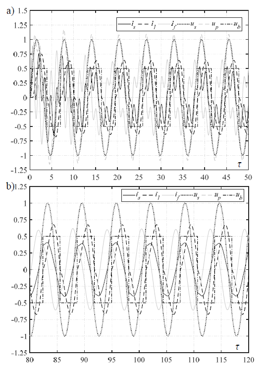
The example waveforms obtained for parameters: cf = 0.5, xs = 0.1, rs = r1 = rf =0.01 and uo = 0.5 are shown in Fig.6a and Fig.6b, respectively for xf = 0 (i.e. without inductance Lf) and xf = 0.2378 (with inductance Lf). Parameter xf was calculated for resonant frequency order nr equal to 2.9. Significantly smaller distortions for waveforms in Fig.6b are observed. Whereas the transients after switching on the supply voltage become longer than for xf = 0. Therefore, obtained waveforms are shown only in steady state, achieved after approx. 13 cycles. The period for the adopted time scale τ is equal to 2π.
The values of THD for analysed waveforms are presented in Table 1. For xf = 0.2378 the THD of current is decreased about ten times compared to xf = 0, whereas for current if approximately four times. The distortion of the voltage up is also much smaller than for xf = 0. The THD of current i1 and voltage ub are practically unchanged.
Table 1. Total harmonic distortion for currents and voltages waveforms in circuit

After taking into account the parameter xf, the power factor PF is also improved at specific points of the analyzed circuit. The values of power factor PF and power factor of fundamental harmonics PF1 are shown in Table 2. These were measured at the voltage source terminals (PFin, PF1in), the PCC point (PFPCC, PF1PCC) and the input terminals of nonlinear load (PFload, PF1load). The power factor PF significant increased for xf = 0.2378 in voltage source VS and PCC point. The power factor of nonlinear load PFload increases slightly. After taking into account parameter xf the power factor of the fundamental components don’t change significantly.
Table 2. The power factor PF and power factor for fundamental components PF1 in different part of circuit

The obtained power factor results are close to unity for the voltage source VS and PCC point. The value of this coefficient for nonlinear load remains practically constant, both when inductance Lf in a circuit occurs or not.
Power distribution in circuit
The distribution of active and reactive power in analysed circuit was carried out in MATLAB/Simulink system. The total active and reactive power were calculated following:

The reactive power was defined as the product of voltage and current time derivative dI/dt and averaged over the period T [2]. The powers (7) may be written as sum of the power of first harmonic component and power of higher harmonics components:
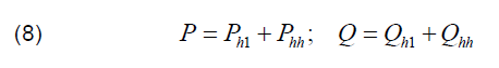
where: Ph1, Qh1 – respectively the active and reactive power of the fundamental component; Phh, Qhh – respectively the active and reactive power of the sum of higher harmonics.
The power distribution in circuit was analysed for total power, first harmonic power and higher harmonics power. Calculating the total powers (P,Q) and the powers of the first harmonics (Ph1,Qh1), the powers of the higher harmonics (Phh,Qhh) may be determined from (8). The power components were referenced to E2s/ꙍL1 and analysed using dimensionless variables. The analyse was carried out for the same parameters as previous section.
Figure 1a shows the distribution of reactive power in circuit for xf = 0. The total reactive power and the power of first harmonic of the voltage source VS are close to zero. This is due to the reactive power compensation in circuit. The total reactive power of nonlinear load NL is also close to zero, whereas the reactive power of the first harmonic and the reactive power of the higher harmonics of this load have similar values, but opposite signs. The reactive power conversion of first harmonic into the reactive power of higher harmonics is observed. Next, the reactive power of higher harmonics of nonlinear load NL is fully transferred to the equivalent reactance of the supply circuit.
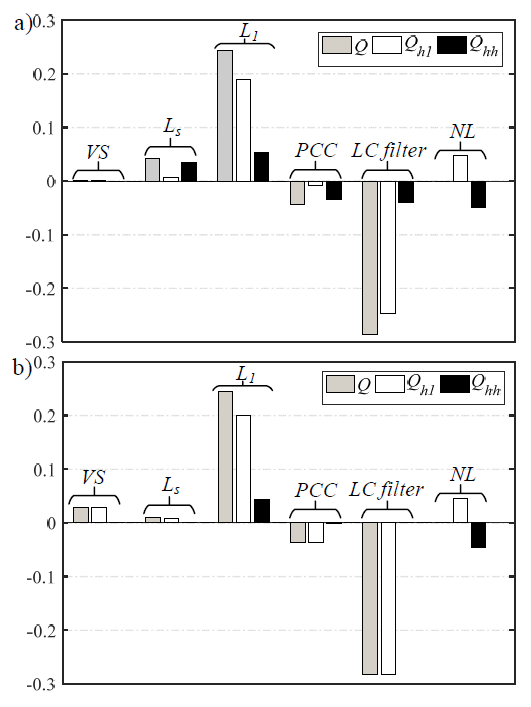
For xf = 0.238 (Fig.7b) the reactive power of higher harmonics at the PCC point, inductance Ls and LC filter decreased. The reactive power of higher harmonics in nonlinear load does not change significantly in compare to xf = 0. Its value is comparable to the reactive power of first harmonic of load and reactive power of higher harmonics of the inductance L1.
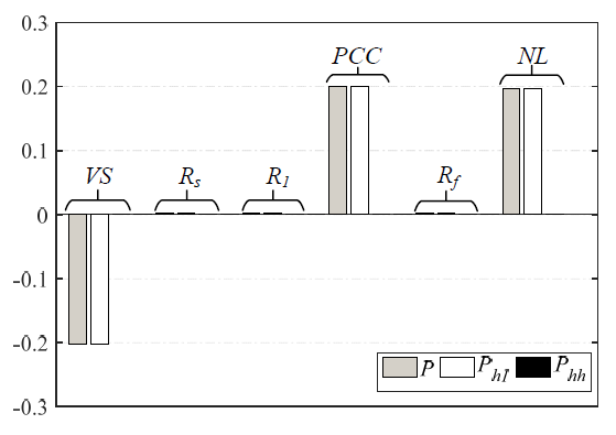
The parameter xf has not a significant influence on active power in circuit. For xf = 0.238 very small changes of active power are observed in compare to xf = 0. Therefore, the distribution of active power shown in Fig.8 concerns only to the case if xf = 0.238. The active power of the higher harmonics on all elements is close to zero. In effect the total active power and the active power of the fundamental harmonic are comparable.
When a capacitor to reactive power compensation is used, the reactive power of higher harmonics increases in the circuit. The reactive power of higher harmonics is dissipated in all parts of circuit, excluding the voltage source, that is sinusoidal. After taking into account inductance Lf, this power is reduced to zero in selected elements and points of circuit. The power of higher harmonics of nonlinear load and inductance L1 remained practically unchanged, even if inductance Lf is used.
Conclusion
The model of circuit with nonlinear load and LC passive filter enabled quantitative analysis of power conversion phenomena and harmonics propagation. The analyses confirm influence of the mains inductance on increase of currents and voltages distortion in circuit.
The analyses indicate need to take into account the additional series inductance for capacitor banks in analysis of power factor and total harmonic distortion in circuit. The inductance of LC passive filter selected for 2.9th harmonic frequency order (in close to 3rd harmonic) allowed to significantly reduce power conversion phenomena occurring in the circuit. This inductance should be also taken into account in the analysis of other higher harmonics.
REFERENCES
[1] Singh B., Chandra A.: Power Quality – Problems and Mitigations Techniques, John Wiley & Sons Ltd, 2015
[2] M. Wciślik: Powers Balances in AC Electric Circuit with Nonlinear Load, IEEE 2010
[3] R. Klempka: Designing a group of single-branch filters taking into account their mutual influence, Archives of electrical engineering, 2014, s. 81 – 91
[4] M. Włas: Engineering design of passive filter structures, Zeszyty Naukowe Wydziału Elektrotechniki i Automatyki Politechniki Gdańskiej Nr 28, s. 143-148, 2010
[5] A. Lange and M. Pasko: Selected methods of improving electrical energy quality with LC systems, Gliwice: Wydawnictwo Politechniki Śląskiej, 2015
[6] C. S. Mboving, Z. Hanzelka and R. Klempka: Different approaches for designing the passive power filters, Przegląd Elektrotechniczny, 11 2015, s. 102-108
[7] IEEE Recommended Practices and Requirements for Harmonic Control in Electrical Power Systems, IEEE Std 519-1992, 15/2004
Authors: Professor Mirosław Wciślik, Kielce University of Technology, Department of Electric Engineering, Automatic Control and Computer Science, al. Tysiąclecia Państwa Polskiego 7, 25- 314 Kielce, E-mail: wcislik@tu.kielce.pl; MSc Paweł Strząbała, Kielce University of Technology, Department of Electric Engineering, Automatic Control and Computer Science, al. Tysiąclecia Państwa Polskiego 7, 25-314 Kielce, E-mail: pstrzabala@tu.kielce.pl
Source & Publisher Item Identifier: PRZEGLĄD ELEKTROTECHNICZNY, ISSN 0033-2097, R. 96 NR 3/2020. doi:10.15199/48.2020.03.14
