Published by Vishnu SURESH, Dominika KACZOROWSKA, Przemyslaw JANIK, Jacek REZMER,
Wroclaw University of Science and Technology
Abstract. This paper deals with load flow analysis of local microgrid containing a stochastic renewable energy source and storage. The study is carried out using the Matpower toolbox with all relevant constraints considered regarding storage, power lines and other components. Certain operational scenarios of the microgrid are also discussed.
Streszczenie. Niniejszy artykuł dotyczy analizy rozpływu mocy w lokalnej mikrosieci zawierającej stochastyczne odnawialne źródło energii i magazynowan energii. Analizę przeprowadzono przy użyciu zestawu narzędzi Matpower ze wszystkimi istotnymi ograniczeniami w odniesieniu do magazynu energii, linii energetycznych i innych komponentów. Omówiono również niektóre scenariusze operacyjne mikrosieci – Analiza rozpływu mocy w lokalnej mikrosieci z magazynem energii
Keywords: Microgrid, Matpower, storage, Renewable energies, Power flow.
Słowa kluczowe: Mikrosieci,, Matpower, magazyn energii, Odnawialne źródła energii, Rozpływ mocy.
Introduction
The increasing penetration of renewable energy sources and restrictions on expansion of centralised conventional sources of power has led to research into microgrids.
Microgrids represent a low voltage system hosting a network of distributed energy sources, storage and loads that is tailored to a local environment [2,4]. The energy is generated close to the areas of consumption thereby reducing transmission and distribution losses incurred on account of longer transmission lines along with multiple environmental benefits.
From the point of view of the system operator the microgrid is seen as a single system [4]. The energy sources in the network are stochastic and the problem of energy balance, load flow and power quality become complex. Hence, this paper presents modelling of microgrids, associated load flow problem and its solution employing a MATLAB toolbox named MATPOWER developed by Cornell University [1].
It describes the decision-making process involved with storage connected to the microgrid. The effect of reactive power compensation on overall power demand on the grid and a few operational scenarios.
Current research in this area includes modelling of local microgrids in simulation packages, such as MATLAB [4] and industrial software such as ETAP[6], Matpower also contains numerous test cases of power system models used for load flow and optimal load flow studies that can be found in [1]; typically most cases are related to conventional power systems not containing renewable or sources of a stochastic nature This paper explores its adaptability regarding sources of stochastic nature, In [4] the focus was laid on two different microgrid cases differing in the number of storage units used and a dynamic approach to modelling storage has been introduced which is being adopted in this study on microgrids. In [6] the modelling of the grid took into account the load demand and had included a wind turbine generator as one of the sources. In the present study the load flow is carried out with storage but is modelled as a local scenario. Numerous other methods exist to solve typical load flow problems that involve solving a set of nonlinear equations, they are discussed in detail in [7,8].
Microgrid Components and load flow problem formulation
The system used in this study is a 4-bus network representing a typical configuration of a microgrid located far from the utility grid, similar to the situation of rural areas. Every bus is characterised using four variables as given below [2,5]:
(1)
• Pi(t) – Active power injected into the bus
• Qi(t) – Reactive power injected into the bus
• Vi(t) – Voltage magnitude at the bus
• δi(t) – Phase angle of the voltage at bus
Here, i = 1,2,…..,n represents the number of buses in the given network.
The utility grid is taken as the reference bus [5], It is common practice since the utility grid in this scenario would be able to provide active and reactive power according to the needs of the microgrid. The voltage magnitude and angle for a reference(slack) bus is always 1∠0o.
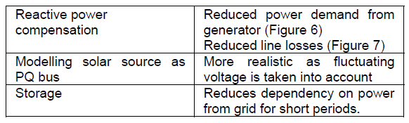
Commonly sources modelled as PV buses [5] have active power and voltage magnitude specified but in reality, solar energy sources exhibit voltage changes during production time, hence, it is more appropriate to model solar sources as a PQ buses as it is done in this study.
Storage is modelled as a PV source [2] and since the time dimension is involved with the operation of storage, a dynamic approach to its modelling is used as described in [2].
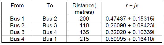
Load is modelled as a PQ bus [5]. Reactive power compensation is provided along with solar source at the bus in order to study its influence on the power supply. The shunt capacitor bank used is a Legrand – Automatic – H Type 3 Phase 400 V-50 HZ -75 KVAR. The distribution lines used in the study are NKT low-voltage IEC standard – 60502-1:2004 lines, as described in the Table 1.
Table 1: Cable data
In this study the data input for solar PV is obtained from in-house solar panels installed at the Wroclaw University of Science and Technology. The load data obtained is real, one week data utilised for study purposes. The utility grid in this study has been taken as a large generator that would be able to supply active and reactive power as per system requirements to carry out power flow analysis.
The power flow problem involves solving for the above mentioned four variables in (1). The equations are given below.
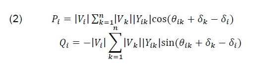
where, i = 1,2,…..,n. Yik – represents self-admittance and mutual admittances and together form the bus admittance matrix which is crucial to obtain values of all parameters at all buses.
Equations (2) represent 2n power flow equations for active and reactive power at all buses and since each bus has 4 variables, the resultant is 4n variables that has to be solved. Since every bus has been assigned a particular bus type, 2 variables are fixed at any given point for a particular bus simplifying the problem to 2n variables. The equations (2) are non-linear algebraic equations, hence it is necessary to apply numerical methods to arrive at a solution [5]. Further information on the theoretical formulation of the problem can be obtained from [5].
There are numerous methods numerous methods available to arrive at a solution for the given problem such as Gauss-Siedel, Newton-Raphson, Fast decoupled load flow methods amongst many others.
In the Gauss-Siedel method, the set of non-linear equations are solved by first assuming a solution vector and by using one of the equations at (2) the revised value of a particular variable is obtained by substituting the other variables in that equation, then the solution vector is updated with regard to this new value. This process is then repeated so as to obtain revised values for all variables and that would complete 1 iteration. This process is then repeated in several iterations until the process converges to a solution with an acceptable accuracy. The gauss Siedel method is considered to be very sensitive with regard to initial solution vector that is chosen [5,10]. If the solution vector chosen is closer to the actual solution then the method will converge faster taking lesser number of iterations, if the solution vector assumed is not accurate then in certain cases the method will fail to converge at a solution.
In order to overcome the issue of performing a large number of iterations in the Gauss-Seidel method, the Newton-Raphson is proposed to solve the set of non-linear equations. [5,10] The Newton-Raphson method is faster at calculating the solution since it is a gradient based solver and the calculation of a Jacobian matrix enables the method to converge on to the solution in a much lesser number of iterations. According to [10] the number of iterations taken for a 500-bus network would be 500 iterations for the Gauss-Seidel method whereas the solution would be arrived in 4 iterations with the Newton-Raphson method. But since the time taken for one iteration is about 7 times in the Newton-Raphson method as in the Gauss- Seidel method the overall gain in speed is about 15 times. Other methods such as the fast decoupled load flow methods further quicken the solution finding process but taking advantage of the weak coupling between (Pi, δi ) and (Qi, Vi) and is typically used in systems consisting of conventional sources of power and long transmission lines[5]. But since, the network used in this study has stochastic sources of energy and shorter distribution lines, the Newton-Raphson method is used for solving power flow equations.
The process involved in running load flow analysis in MATPOWER and the decision-making process involved in storage working is described in a flow chart in Fig. 1
The single line diagram of the setup is as shown in Fig 2. The specifications of all components are also shown. Nominal voltage of the system is 400V.

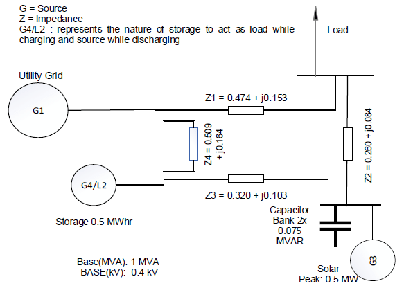
Table 2: Component constraints
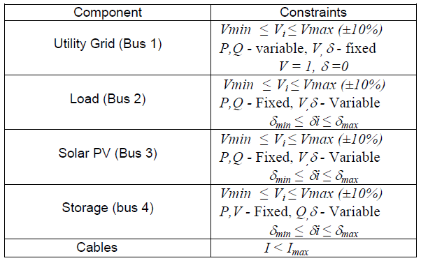
In order to match reality as close as possible all components are subject to constraints that are imposed upon by the hardware itself, type of bus and relevant standards.
Case study results and analysis
The main purpose of load flow is to balance active and reactive power demand and generation as given by the equations below.

where PG, QG, PD, QD, PL, QL represent active power generated, reactive power generated, active power demand, reactive power demand, active power loss in the system and reactive power loss in the system, respectively. Figure 3 is a representation of the equations at (3) and it is evident that active and reactive powers consumed and generated match each other hence validating the accuracy of MATPOWER and the simulated system design.
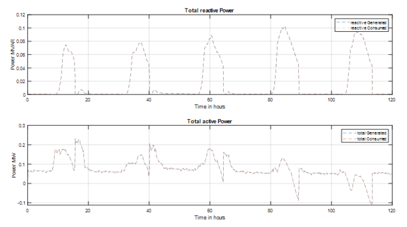

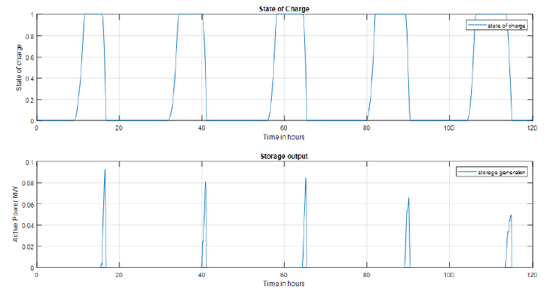
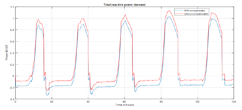
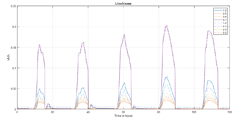
Figure 4 represents the active power output of the solar PV installation, the active power taken in or exported out to the utility grid and the storage capacity. It is inferred from the plots that initially when the solar PV installation is not producing active power all of the load’s demand is met by the grid and also the storage at this time when it is empty. Later on, during mid-day when solar production increases and reaches peak capacity the load is catered to by the solar PV output and excess is used to charge the storage. Since only a part of the energy can be used to charge the storage at any given point of time, the rest of the energy is exported out to the grid. It is seen that when solar output roughly exceeds the load demand and power is being exported to the grid, the storage device starts to charge. Then, when the solar power output reduces and is smaller than the load demand the storage device comes online and produces power for a short while until it is discharged to a threshold level of 10% of storage capacity.
Figure 5 demonstrates how SOC (state of charge) of the storage device changes with its output and storage capacity. From the Fig. 5 it can be noticed that when the storage output generation increases the state of charge value decreases accordingly.
Numerous devices that are connected to the power system tend to draw reactive power from the sources. High demand for reactive power from the loads cause power quality issues such as voltage fluctuations, increased power losses over lines and also increased MVA demand from sources [9].
Nowadays, when the demand for electricity keeps increasing, utilities are faced with the problem of meeting the demand at lower costs. Hence, it has become common practice for the utilities to place compensation devices along the network to manage demand on the network and to improve voltage profiles.
Many techniques are available for the purpose of compensation, some of them being usage of capacitor banks, static var compensators, synchronous condensers, STATCOMs amongst other many others. They are discussed in detail in [9] with standard models.
Figure 6 makes a comparison of the reactive power demand from the grid with capacitor bank connected and disconnected from the bus. It can be seen that the demand for reactive power is higher without compensation than with compensation. This is because a part of the reactive power demand is provided by the capacitor bank.
Figure 7 represents line losses for cases with and without reactive power compensation. It is evident from the figure that the line losses with reactive power compensation (dashed lines) are lower when compared to the line without compensation (solid lines) for lines ‘1-2’ and ‘1-4’ which are the lines used to export and import power from the utility grid, hence it can be concluded that with reactive power compensation overall reactive power demand is reduced.
Table 3: Summary of findings
Conclusions
The study represents a typical microgrid with data that is taken from the real world. Load flow study performed for the network reveals the characteristics with regard to the working of storage and the benefits of localised reactive power compensation. The active and reactive power demand and supply within the network is balanced accurately even though the solar PV and storage system produce energy intermittently and not in a regular manner such as thermal power plants. Moreover, it has been shown that power flow studies can be carried out successfully even when the solar PV source is modelled as PQ bus instead of a PV bus and thus taking into account the fluctuating nature of the solar system voltage.
Further study on the model would be to diversify the sources in the system and carry out optimal power flow using an appropriate optimization technique. Also comparison of the usage of different types of battery storage devices and incorporation of their charging characteristics could be implemented in future studies.
REFERENCES
[1] R. D. Zimmerman, C. E. Murillo-Sanchez, and R. J. Thomas,\Matpower: Steady- State Operations, Planning and Analysis Tools for Power Systems Research and Education,” Power Systems, IEEE Transactions on, vol. 26, no. 1, pp. 12{19, Feb. 2011. DOI: 10.1109/TPWRS.2010.2051168
[2] Yoash Levron, Josep M. Guerrero, Member, IEEE, and Yuval Beck: Optimal Power Flow in Microgrids With Energy Storage. IEEE TRANSACTIONS ON POWER SYSTEMS, VOL. 28, NO. 3, AUGUST 2013.
[3] Chris Marnay, F Javier Rubio, and Afzal S Siddiqui: Shape of the Microgrid, Ernest Orlando Lawrence Berkeley National Laboratory.
[4] S. Abu-Sharkha,1, , R.J. Arnolde,1, J. Kohlerd,1, R. Lia,1, T. Markvarta,*,1, J.N. Rossb,1, K. Steemersc,1, P. Wilsonb,1, R. Yaoc,1. Can microgrids make a major contribution to UK energy supply?
[5] DP Kothari, IJ Nagrath: Modern Power System Analysis, Third edition.
[6]. Sneha Kulkarni, Sunil Sontakke: Power System Analysis of a Microgrid using ETAP , International Journal of Innovative Science and Modern Engineering (IJISME) ISSN: 2319-6386, Volume-X, Issue-X
[7] V. Del Toro, Electric Power Systems. Englewood Cliffs, NJ,USA: Prentice-Hall, 1992, vol. II.
[8] N. P. Padhy, “Unit commitment—A bibliographical survey,” IEEE Trans. Power Syst., vol. 19, no. 2, pp. 1196–1205, May 2004.
[9] J. Nyangoma, K. Awodele* COMPARISON OF DIFFERENT REACTIVE POWER COMPENSATION METHODS IN A POWER DISTRIBUTION SYSTEM Department of Electrical Engineering, University of Cap
[10] Stott, B. (1974). Review of Load-Flow Calculation Methods. Proceedings of the IEEE, 62(7), 916–929. https://doi.org/10.1109/PROC.1974.9544
Authors: Vishnu Suresh, PhD candidate – Wroclaw University of Science and Technology, Faculty of Electrical Engineering, Wybrzeze Wyspianskiego 27,50-370 Wroclaw, E-mail: vishnu.suresh@pwr.edu.pl; Dominika Kaczorowska, PhD candidate – Wroclaw university of science and Technology, Faculty of Electrical Engineering, Wybrzeze Wyspianskiego 27,50-370 Wroclaw, E-mail: dominika.kaczorowska@pwr.edu.pl, dr hab. inż. Przemyslaw Janik – Wroclaw University of Science and Technology, Faculty of Electrical Engineering, Wybrzeze Wyspianskiego 27,50-370 Wroclaw, E-mail: przemyslaw.janik@pwr.edu.pl , dr hab. inż. Jacek Rezmer – Wroclaw University of Science and Technology, Faculty of Electrical Engineering, Wybrzeze Wyspianskiego 27,50-370 Wroclaw. jacek.rezmer@pwr.wroc.pl.
Source & Publisher Item Identifier: PRZEGLĄD ELEKTROTECHNICZNY, ISSN 0033-2097, R. 95 NR 9/2019. doi:10.15199/48.2019.09.19
