Published by Paweł KOWALSKI, Robert SMYK, Gda ´nsk University of Technology
Abstract. The article presents an overview of the thresholding algorithms. It compares the algorithms proposed by Pun, Kittler, Niblack, Huang, Rosenfeld, Remesh, Lloyd, Riddler, Otsu, Yanni, Kapur and Jawahar. Additionally, it was tested how the tuning of the Pun, Jawahar and Niblack methods affects the thresholding efficiency and proposed a combination of the Pun algorithm with a priori algorithm. All presented algorithms have been implemented and tested for effectiveness in detecting overhead lines.
Streszczenie. W artykule przedstawiono przegl ˛ad algorytmów progowania. Porównano w nim algorytmy zaproponowane przez Puna, Kittlera, Niblacka, Huanga, Rosenfelda, Remesha, Lloydaa, Riddlera, Otsu, Yanni, Kapura i Jawahara. Dodatkowo przetestowano, jak dostrajanie metod Puna, Jawahara i Niblacka wpływa na skuteczno ´s ´c progowania oraz zaproponowano poł ˛aczenie algorytmu Puna z algorytmem a priori. Wszystkie przedstawione algorytmy zostały zaimplementowane i przetestowane pod k ˛atem skuteczno ´sci w wykrywaniu linii napowietrznych
Keywords: thresholding, power lines, image processing
Słowa kluczowe: progowanie, linie elektroenergetyczne, przetwarzanie obrazu
Introduction
Modern energy infrastructure is a very complex system prone to failures that should be detected and removed as soon as possible. The construction of the entire infrastructure is characterized by the presence of concentrated elements, e.g. power plants or switching stations. A significant part of the discussed infrastructure are power junkies and transmission lines which is distributed. A critical problem is monitoring and maintaining the efficiency of transmission lines [1, 2, 3]. Technological progress forces the automatic control of monitoring processes. Therefore, techniques for assessing the efficiency of transmission lines based on image processing are implemented. The image can be acquired with a camera installed in an unmanned aerial vehicle (UAV) moving along the line. The problem discussed in this paper concerns image processing to detect power cables in the video stream. The scheme for extracting objects when processing an image frame is often similar. In the initial stage, called preprocessing, edge operators and semgentation algorithms are used. Processing efficiency at this stage is crucial and has a general impact on the efficiency of subsequent processes such as object detection.
This paper focuses on the analytical evaluation of thresholding methods in terms of their application in the monitoring system of power lines from a mobile carrier. The prototype of such a system was elaborated and implemented as part of previously research [4, 5, 6, 7]. One of the important research stages was the validation of thresholding methods as shown in this study. The first section presents the binarization. The next presents the measures used in the threshold selection algorithms. These measures are used in the formulas presenting the operation of individual algorithms in the third chapter. The fourth section presents the procedure for determining the effectiveness of the algorithm. And in the section five the results are discussed.
The basis of image binarization
Edge extraction is the first step in the procedure of detecting the objects in an image. Convolution with edge detection operator results in image Z, where pixel z contains the gradient value. To reduce the amount of data and extract the edges, the segmentation is performed. This procedure relies on dividing an image into disjoint regions characterized by the uniformity of pixel values. The binarization performed as a thresholding procedure is a simplest variant of segmentation. For a given threshold, the pixels below the threshold are considered to form an object (edges) in the image, while the remaining pixels constitute the background. The thresholding algorithm is as follows
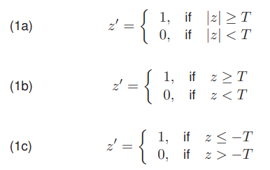
where T indicates the selected threshold value, z represents a pixel of thresholded image, and z is the pixel value of the image resulting from the thresholding, where 1 represents edge and 0 background. (1a) specifies a thresholding without recognizing gradient direction, (1b) specifies a thresholding extracting edges with positive gradient, and (1c) specifies a thresholding extracting edges with negative gradient. The most of popular methods of selecting a threshold value are using a histogram that represents the brightness distribution of the pixels in an image. A histogram is defined as a set of discrete values H = [h0, h1, h2, …, hn]. The individual values of hi are determined by
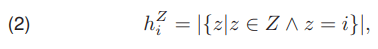
where hZi is a single element of the histogram HZ, i is the index of the element, Z is the image for which the histogram is created. In practice, the value of hZi denotes the number of z pixels whose values are equal to i.
By using the historgram, it is possible to determine the probability distribution of selected pixel values in an image
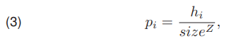
where pi is the probability of occurrence in the image Z a pixel value of i, sizeZ is total number of pixels in the image Z, and hi is the number of pixels with a value i. We founded, that as a result of image segmentation, the background class and the graphical object class are obtained. A known method of determining the probability of occurrence of a pixel belonging to one of the mentioned classes may be used
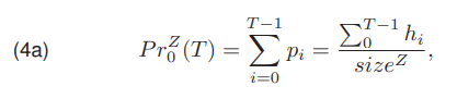

The probability of a pixel belonging to the background class PrZ0 (T) (4a) is the sum of the probabilities of all pixels belonging to the background class. Likewise, the probability of a pixel belonging to an object class PrZ1 (T) (4b) is the sum of the probabilities of all pixels belonging to the object class.
Another measures are the arithmetic mean of the pixel values of an image SrZ, average value of pixels belonging to the background class SrZ0 (T) and to the class of the object SrZ1 (T)
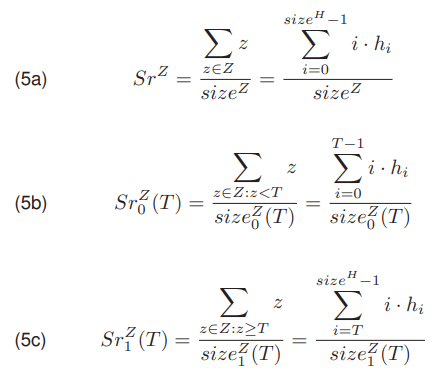
where sizeZ0 (T) and sizeZ1 (T) denotes the number of pixels belonging to the background class and the object class in Z, respectively. A values of the SrZ (5a), SrZ0 (T) (5b) and SrZ1 (T) (5c) can be determined directly from the image Z or using a histogram H.
Using the measures formulated above we get the variances (6) that are determined by

where σ2Z (6a) is the variance of image Z, σ2Z,0(T) (6b) is the variance of the background class and σ2Z,1(T) (6c) is the variance of the object class. Additional measure used in the thresholding algorithms is Shannon entropy Sh(pr) [8], which is identified by

where pr denotes probability. In the case of splitting the image into two classes, pr and 1 − pr denotes the probability of the pixels belonging to one class or the other, respectively. Additionally, the course of the function Sh(pr) is monotonically increasing in (0; 0, 5) and decreasing monotonically in (0, 5; 1).
Review of the threshold selection methods
This section discusses the threshold selection algorithms used in the later experimental work involving the development of a complete method for the detection of power line conductors. Using a priori knowledge in the thresholding algorithm requires the size of the object estimation. For estimation of the number of pixels representing the shape of power conductors we assumed a horizontal orientation. This means that the pixels of such an line lie on all the columns of the image. Additionally, the shape of power cables is composed of two edges, each one pixel wide. The wire in the image has an opposite gradient at the top and bottom. We can estimate the number of edge pixels using a formula
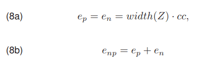
where cc denotes the number of wires visible in the image Z, width(Z) is the width of this image, ep and en is the number of edge pixels with positive and negative gradients, respectively and enp is the estimated number of all edge pixels in the image Z. The a priori algorithm works by setting the threshold T as high as possible, but in such a way that the number of pixels assigned to the object class is greater than or equal to the estimated number of edge pixels. Another method was proposed by Niblack [9], where the threshold value is determined as the sum of the mean SrZ and the square root of the variance σ2Z multiplied by the coefficient Nibk
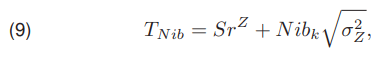
where Nibk is a constant value coefficient Nibk = −0, 2.
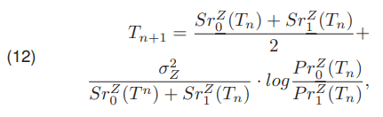
Among the threshold selection algorithms, there are a number of iterative algorithms, where next value of the threshold Tn+1 using the current threshold value Tn is calculated in repeated iterations. The procedure can be carried out until the threshold value stabilizes at the desired level E, which is an absolute error |Tn+1 − Tn| < E. However, there may be cases where the threshold value will oscillate between a few close values and consequently the average of these values is determined.
The algorithm starts with a fixed initial value T0, which should be selected. Thus, initiating the algorithm with a start value close to the final threshold gives a small number of iterations necessary to stabilize the threshold value.
One of the popular iterative methods was developed by Riddler and Calvard [10]. The algorithm should be initialized with a threshold value representing the background, which corresponds to T0 = 1. If the object occupies less than half of the image the initial threshold value has to be calculated as the average value of all image pixels (10).

The threshold update is carried out by (11)
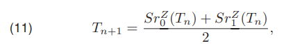
where Tn is in the current and Tn+1 in the next step threshold value.
The Lloyd method [11] is another representative of the iterative approach. The calculations are performed by
The variables in the relationship were described earlier. Another method used in the work is the iterative algorithm proposed by Yanni [12]. The initial threshold value T0 is
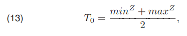
where minZ denotes the minimum value of the pixel present in the image Z, and maxZ maximum value. Each iteration in the discussed approach is carried out by
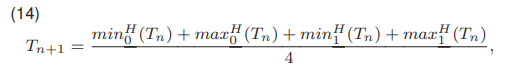
where minH0 (Tn) is the id of minimum histogram value belonging to the background class, maxH0 (Tn) is the id of maximum histogram value of the background class, minH1 (Tn) is the id of minimum histogram value of the object, and maxH 1 (Tn) specifies the id of maximum histogram value of an object class in the image Z. It has been noticed that in the case of power cables detection, in most cases the algorithm termination condition is reached after three iterations. The algorithm mentioned above has a low computational cost because the threshold is determined using the average of four values.
The Rosenfelda method [13] is based on the geometric analysis of the histogram. The histogram H can be represented graphically as a Cartesian bar graph (Fig. 1), where the tops of the bars have coordinates (i, hi). The first step in this method relies on finding the shortest polyline Ħ that lies on above the histogram H and connects its extreme ends. The shape of the Ħ polyline tracing the histogram can be written as a set of vertices. Next, the place where the H histogram is the farthest from the polyline Ħ is sought.
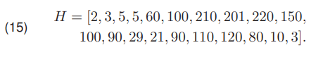
In (15) a vector of example values representing the histogram is presented. For the histogram H (15), a polyline Ħ (16) was created

where each point represents the vertex of the polyline Ħ. The graphic representation was shown on (Fig. 1). The final
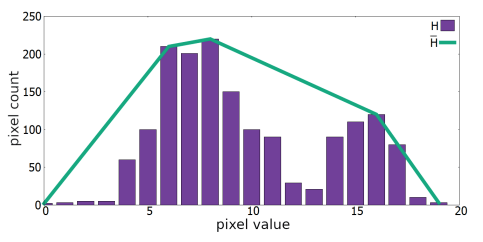
step in Rosenfeld’s algorithm is to find the bar of H that is furthest from the polyline Ħ, which is h12 visible on Fig. 1.
A separate group of threshold selection methods used here are optimization algorithms. They work by finding the minimum or maximum of the goal function. One of such methods is the Otsu algorithm [14, 15], in which the selection of the threshold for dividing the image into two classes is carried out by minimizing the variance for each class. The algorithm works by selecting a threshold with the lowest intra-class variance σ2wew
Determining the intra-class variance is difficult. The formula for the inter-class variance σZmie(T) is simpler
The relationship between the global variance σ2Z, the inter-class variance σZmie(T) (18), and the intra-class variance σ2wew(T) (17) is as follows
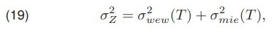
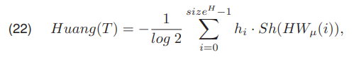
where σ2Z (19) is a constant value, independent of the selected threshold T. It can be seen that minimizing the intra-class variance is equivalent to maximizing the inter-class variance. Calculating the inter-class variance is less computationally complex and is faster. Therefore, the threshold should be calculated by maximizing the inter-class variance. The Huang and Wang algorithm [16] is another thresholding method from the optimization group. It is based on the use of the membership function HWμ(z) represented by
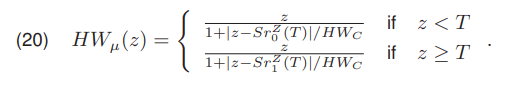
The value of the function HWμ(z) for any pixel z should be within the range from 0.5 to 1. The coefficient value HWC is carried out using

where max(Z) is the maximum pixel value in the image Z, and min(Z) the minimum pixel value present in the image Z. The threshold value in Huang’s method is determined by minimizing the objective function Huang(T)
Jawahar, Biswas and Ray in [17] presented a method in which the threshold is selected by minimizing the mean square objective function Jaw(T) expressed as

where Jawτ denotes the amount of blur between the background and object classes in the image Z. This value has a key influence on the effectiveness of thresholding. According to [17] this argument should be Jawτ ≥ 1. The value of Jawτ = 1 corresponds to the k-means algorithm [15].
Kittler and Illingworth [18, 19] presented a method in which the threshold is selected by minimizing the function Kittler(T) expressed by (24)
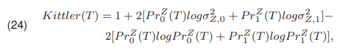
By using the function Sh shown in (7) the equation (24) can be written as (25):

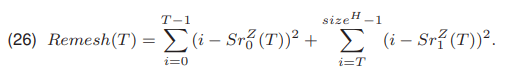
The method proposed by Remesh [20] is based on the minimization of the function Remesh(T) (26)
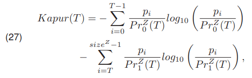
On the other hand, Kapur presented a method [21] in which the threshold is selected by maximizing the function Kapur(T) (27)
Pun [22] presented another optimization method. Using the formula developed by Shannon [8] he defined four entropies, and using them he defined the function PunFe(P unα) (28)
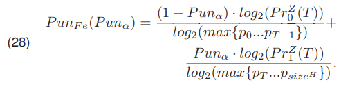
Pun in [22] proposed to search for a threshold T, by minimizing the function PunFe(P unα) On the other hand, Kapur in [21] proposed to determine the threshold T by maximizing the function PunFe(P unα).
In another work, Pun [23] proposed to search for the optimal threshold using an anisotropic coefficient, hereinafter referred to as Punβ. To determine this coefficient, it is necessary to estimate the smallest threshold T0, which divides the histogram into two parts, the first of which should contain at least half the pixels. The initial threshold may be estimated as

and next T0 is used to calculate the anisotropic coefficient Punβ (30)

Then the coefficient Punβ is used to determine the threshold value using the relationship
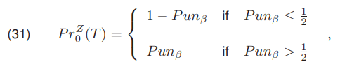
In the case of Punβ > 1/2 a probability PrZ0 (T) equal Punβ and in the case of Punβ ≤ 1/2 the provability PrZ0 (T) should equal 1 −Punβ.
Both Pun algorithms showed low efficiency in detecting the edges of overhead wires. This is because they are specialized in thresholding images to recognize text, where typically the pixel count of the object class is close to the pixel count of the background class. In the case of overhead lines, the difference in the number of pixels of each class is significant. Typically, the number of pixels representing wire edges does not exceed 1% of total pixels.
In order to adapt the second Pun algorithm to detect power line conductors, the formula (29) has been replaced by the formula

where the factor Punmod was introduced, which specifies the initial ratio of the number of pixels of the object class to the number of pixels of the background class.
The next modification is to determine the initial threshold T0 using the formula (8a) from the a priori method. Then Punβ is determined by using (30) and tuned up by coefficient apβ. The selection of the T treshold is done by minimizing the function apPun(T)

Effectiveness of thresholding algorithms comparison
The effectiveness analysis of the threshold selection algorithms was made using a representative set of photos of overhead wires. The pixels representing the wire in each photo were predetermined. The illustration of original picture and selected pixels are on Fig. 2. The function efi(x) has been defined and using the following formula for the effectiveness of detection of the i-th conductors in the column x was established
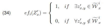
where, ~Wix stands for the set of pixels representing the i-th wire in the pixel column x, and z’x,y is the (x,y) pixel value of the image after edge extraction. The measure of effectiveness effbw is formulated as the sum of the measures efi(x) for all lines in all columns of the image
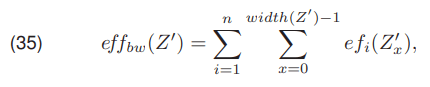
where n determines the number of visible wires, and width(Z’) is the image Z width. Additionally, the relative efficiency effww expressed by (36) determines the percentage number of detected columns

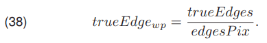
After the image has been processed using the edge detection and thresholding algorithm, the pixel counts can be determined as follows
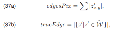
where edgesPix (37a) is the total number of pixels detected as the edge, and trueEdges (37b) the number of edge pixels that represent a correctly detected wire edge. With the use of the presented dependencies on the number of pixels, the coefficient trueEdgewp (38) was formulated. It denoting the number of correctly detected edge pixels in relation to all detected edge pixels
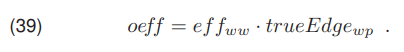
The coefficients were used to elaborate a general measure of the algorithm’s effectiveness in wire detection oeff, which is expressed as
In the initial phase of the research on the development of a complete overhead cable detection procedure, the algorithms discussed in this paper were implemented and validated. First the software environment was used for verification of all the methods, and next the most effective methods are implemented in hardware FPGA environment. The validation was carried out using a set of photos of overhead lines taking into account the typical range of possible combinations of the location of the objects in the image against the environmental background.
Results discussion
The presented algorithms are implemented and used in the image processing procedure. It consists of image conversion to grayscale, convolution with the horizontal mask of Sobel operator [24, 4], selection of the threshold with the selected method and binarization. Then, the detection efficiency of overhead wires using this procedure was determined as oeff (39).
Several of the presented threshold selection algorithms have coefficients whose value can be fine tuned. These are the Jawahar algorithm, the second Pun algorithm with modifications, and the Niblack algorithm. The tuning of the values of the coefficients contained therein on the effectiveness of wire detection has been tested. The tests were performed using the thresholds (1a), (1b) and (1c) for the given image sets, respectively OPKnp, OPKp and OPKn.
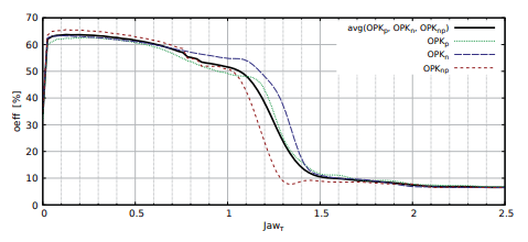
The results of the Jawahar method effectiveness tests are presented on Fig. 3. The influence of the coefficient Jawτ on oeff was shown. The maximum effectiveness of oeffavg = 63, 5% of the Jawahar method is obtained for Jawτ = 0, 13. The effectiveness above 50% is reached forJawτ ∈ (0, 01; 1).
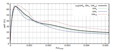
For the second Pun algorithm, the influence of the coefficient Punmod on the effectiveness of thresholding oeff was analyzed and shown on Fig. 4. Thresholding with Punmod > 0, 005 have the efficiency oeff < 25%. After choosing the appropriate value Punmod a significant improvement is obtained over the classical implementation of the second Pun method. Highest efficiency is achieved by modification Punmod (32) on the level of oeffavg = 65% for Punmod = 0, 00029. Modification of the coefficient Punmod by setting a constant value close to 0, increased the effectiveness of thresholding compared to the unmodified version of the algorithm.
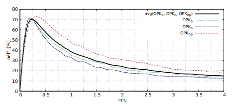
On a Fig. 5 a results of thresholding effectiveness tests using of the second Pun algorithm combined with a priori was shown. It should be noted, that the effectiveness of the thresholding oeff is dependent on the value of the coefficient apβ. Fig. 5 illustrate the results showing the dependence of the apβ coefficient on the effectiveness of thresholding oeff. For apβ ∈ (0, 16; 0, 46) combination of a priori and Pun2 method reaches the effectiveness oeffavg above 60%. The maximum value of oeffavg = 70% is achieved for apβ = 0, 26.
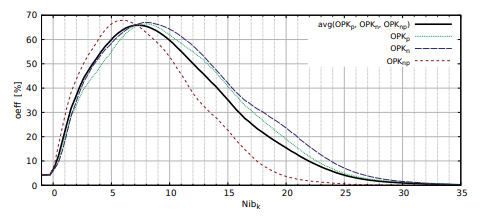
In the classic version of the Niblack method used for the segmentation of images containing text, the coefficient Nibk is a constant −0, 2 [9]. The influence of modifying Nibk for effectiveness oeff of Niblack algorithm in detection of overhead wire edges was checked. The results of the tests are on Fig. 6, where the effectiveness of wire detection oeff (39) depending on the value of Nibk was shown. The effectiveness oeffavg above 60% is achieved for Nibk ∈ (5, 9; 8, 5). However, the maximum overall efficiency of the algorithm oeffavg = 66%, for the test set is obtained with Nibk = 7, 2. In order to check the maximum possible effectiveness, an analysis of the photos used to test the thresholding algorithms was carried out. The experiment consisted in checking all possible thresholds for each photo. For each image the threshold was individually selected to meet maximum oeff. The oriented algorithm is based on expert knowledge, so it cannot be implemented in a real image processing system. After analyzing the entire set of photos for that case, the maximum possible effectiveness of the threshold was determined on oeffavg = 74, 5%.
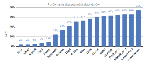
The overall test results are shown on Fig. 7 as an average measure of the effectiveness of wire detection oeffavg for each of the tested algorithms. The effectiveness of the tested algorithms has the values from 4% to 66%, and about half of the tested algorithms achieve effectiveness over 50%. The three most effective algorithms among the tested are modified by authors versions of known methods, which were not intended for wire detection. In this case the classic versions achieve efficiency below 10%. Summing up, the validated algorithms was divided into three basic groups:
• optimization — their point is to minimize or maximize the appropriate function. Its argument is usually the T threshold. These algorithms include: algorithms Jawahar, Kapur, Otsu, Huang, Kittler, Remesh, Pun1 and Pun2,
• iterative — their operation is based on a repeated calculations. The experiments shows that these algorithms usually require several steps to achieve the satisfactionary result. Representatives of such algorithms are Yanni, Riddler oraz Lloyd,
• algorithms running in place — in which the calculation procedure is one-shot, they include algorithms marked as Niblack and a priori
The most computationally expensive and time consuming are optimization algorithms. Iterative algorithms have less computational effort due to the relatively small number of steps. It should be mentioned that, for example, in processing a video stream, the threshold calculated in the previous frame can be passed as the initial value of T0 in present processed frame. In this case, stabilization usually does not exceed three iterations. The fastest and the most predictable in terms of runtime are one-shot algorithms. It is a tuned version of the Niblack method and the a priori method, which achieved efficiency of 66% and 61% respectively. In this case, the distribution of pixel values in the image does not noticeably affect the execution speed of the algorithm. The presented advantages cause that, these algorithms are suitable for transfer to the FPGA environment.
Conclusion
In the paper an analysis of the threshold selection algorithms intended for image segmentation was shown. These algorithms were appraised for their usability in detecting overhead lines. The selected algorithms have been implemented in a mobile non-contact monitoring system. Image processing and wire detection are a key component of this system. The analysis of the selection of the threshold value carried out in this work and the presented measures of effectiveness were used in the development of the mentioned monitoring system.
The performance of cable detection was compared using the measure oeff prepared by the authors. Among the tested algorithms, optimization, iterative and in-place algorithms can be distinguished. A total of 17 threshold selection methods were tested. In addition, an expert-based algorithm was developed that determined the maximum cable detection efficiency of 75%. The highest efficiency 66% was achieved by two methods, the Niblack and the second Pun method combined with the a priori method. The Pun method is an optimization algorithm. Its implementation requires a high computational effort. Whereas the Niblack method is computationally simpler because it is an in-place (one-shot) algorithm. This leads to the conclusion that this algorithm can be used in a hardware implementation of a real-time image processing system.
REFERENCES
[1] W. Doł ˛ega, “Bezpiecze ´nstwo pracy krajowych sieci dystrybucyjnych,” Przegl ˛ad Elektrotechniczny, vol. 96, pp. 21–24, 2020.
[2] W. Doł ˛ega, “Awarie krajowych linii napowietrznych–wybrane aspekty,” Przegl ˛ad Elektrotechniczny, vol. 97, pp. 9–14, 2021.
[3] T. Tambi, “Real-time monitoring of high voltage insulators in the tropical climate,” Przegl ˛ad Elektrotechniczny, vol. 96, pp. 129– 135, 2020.
[4] P. Kowalski, Application of image processing methods for overhead power lines monitoring. PhD thesis, Gdansk University of Technology, 2020. (in Polish).
[5] P. Kowalski, M. Czy ˙zak, and R. Smyk, “Comparison of edge detection algorithms for electric wire recognition,” in ITM Web of Conferences, vol. 19, p. 01044, EDP Sciences, 2018.
[6] P. Kowalski and M. Czy ˙zak, “High voltage line distance measurement and position detection based on stereoscopic image,” in 2018 International Interdisciplinary PhD Workshop (IIPhDW), pp. 54–57, May 2018.
[7] P. Kowalski and R. Smyk, “Overhead wires detection by fpga real-time image processing,” in ITM Web of Conferences, vol. 28, p. 01046, 2019.
[8] C. E. Shannon, “A mathematical theory of communication,” Bell system technical journal, vol. 27, no. 3, pp. 379–423, 1948.
[9] W. Niblack, An introduction to digital image processing. Strandberg Publishing Company, 1985.
[10] T. Ridler and S. Calvard, “Picture thresholding using an iterative selection method,” IEEE Transactions on Systems, Man, and Cybernetics, vol. 8, pp. 630–632, Aug 1978.
[11] D. Lloyd, “Automatic target classification using moment invariant of image shapes,” IDN AW126, RAE, Farnborough, Reino Unido, 1985.
[12] M. Yanni and E. Horne, “A new approach to dynamic thresholding,” in EUSIPCO’94: 9th European Conf. Sig. Process, vol. 1, pp. 34–44, 1994.
[13] A. Rosenfeld and P. De La Torre, “Histogram concavity analysis as an aid in threshold selection,” IEEE Transactions on Systems, Man, and Cybernetics, vol. SMC-13, pp. 231–235, March 1983.
[14] N. Otsu, “A threshold selection method from gray-level histograms,” IEEE Transactions on Systems, Man, and Cybernetics, vol. 9, pp. 62–66, Jan 1979.
[15] A. Wodoła ˙zski, “Wybrane algorytmy uczenia maszynowego w segmentacji obrazu kłaczków osadów ´sciekowych,” Przegl ˛ad Elektrotechniczny, vol. 97, pp. 134–136, 2021.
[16] L.-K. Huang and M.-J. J. Wang, “Image thresholding by minimizing the measures of fuzziness,” Pattern recognition, vol. 28, no. 1, pp. 41–51, 1995.
[17] C. Jawahar, P. K. Biswas, and A. Ray, “Investigations on fuzzy thresholding based on fuzzy clustering,” Pattern Recognition, vol. 30, no. 10, pp. 1605–1613, 1997.
[18] J. Kittler and J. Illingworth, “Minimum error thresholding,” Pattern recognition, vol. 19, no. 1, pp. 41-47, 1986.
[19] H. Yan, “Unified formulation of a class of image thresholding techniques,” Pattern Recognition, vol. 29, no. 12, pp. 2025–2032, 1996.
[20] N. Ramesh, J. . Yoo, and I. K. Sethi, “Thresholding based on histogram approximation,” IEE Proceedings – Vision, Image and Signal Processing, vol. 142, pp. 271–279, Oct 1995.
[21] J. N. Kapur, P. K. Sahoo, and A. K. Wong, “A new method for gray-level picture thresholding using the entropy of the histogram,” Computer vision, graphics, and image processing, vol. 29, no. 3, pp. 273–285, 1985.
[22] T. Pun, “A new method for grey-level picture thresholding using the entropy of the histogram,” Signal processing, vol. 2, no. 3, pp. 223–237, 1980.
[23] T. Pun, “Entropic thresholding, a new approach,” Computer graphics and image processing, vol. 16, no. 3, pp. 210–239, 1981.
[24] I. Sobel and G. Feldman, “An isotropic 3×3 image gradient operator. stanford artificial intelligence project (sail),” 1968.
Authors: Ph.D. Paweł Kowalski, Ph.D. Robert Smyk, Department of Electrical and High Voltage Engineering, Faculty of Electrical and Control Engineering, Gda ´nsk University of Technology, ul. Gabriela Narutowicza 11/12 80-233 Gda ´nsk, Poland, email: pawel.kowalski@pg.edu.pl, robert.smyk@pg.edu.pl
Source & Publisher Item Identifier: PRZEGL ˛ AD ELEKTROTECHNICZNY, ISSN 0033-2097, R. 98 NR 3/2022. doi:10.15199/48.2022.03.34
