Simplified Formula for the Load Losses of Active Power in Power Lines taking into Account Temperature

Published by Stanislav S. GIRSHIN, Oleg V. KROPOTIN, Vladislav M. TROTSENKO, Aleksandr O. SHEPELEV, Elena V. PETROVA, Vladimir N. GORYUNOV, Omsk State Technical University, Omsk, Russia

---

Abstract. The use of a simplified formula for calculation of active power losses in transmission lines taking into account the temperature in the stationary thermal regime is considered. The results of the comparison of losses calculated using a simplified formula and based on the solution of the full heat balance equation for wires of various types are presented. The dependences of the calculating errors on the load current with and without solar radiation are constructed and analyzed.

Streszczeni. W artykule rozważa się korzystanie z uproszczonej formuły do obliczania strat mocy czynnej w linii z uwzględnieniem temperatury w trybie stacjonarnym cieplnym. Straty oblicza się według uproszczonego wzoru i w oparciu o równania bilansu cieplnego dla przewodów różnych typów. Zbudowane są i analizowane zależności błędów obliczeń od prądu obciążenia z promieniowania słonecznego i bez niego. Uproszczone zależności do obliczania strat mocy czynnej w linii z uwzględnieniem temperatury

Keywords: bare and insulated wires, energy losses, temperature.
Słowa kluczowe: gołe i izolowane przewody, straty energii, temperatura.

Introduction

Load losses of energy in power lines account for about 85% of the total losses in the lines and about 55% of the total losses in the electrical networks of Russia. Improving the efficiency of power transmission imposes rather high demands on the accuracy of the calculation of losses. This in turn leads to the necessity of taking into account all the main factors determining the amount of losses. One of these factors is the temperature dependence of active resistance [1-3].

The papers in the field of accounting for the temperature of wires in the calculation of energy losses in electrical networks are rather popular nowadays [4-8]. However, the relevant methods are not widespread, in addition to the standards presented in [9-10]. For example, modern programs for calculating energy losses usually take into account only the dependence of active resistances on the ambient temperature, but not heating by current. The main reason for this is that a fairly large amount of additional input data is required to accurately calculate the temperature.

The problem can be formulated as follows: it is required to develop such methods for calculating energy losses, which would take into account both the ambient temperature and the heating of the wires by the load currents, but would require a minimum amount of source data.

In this article, a simplified formula for heat loss is compared with more complex methods.

Basic equations and formulas

In the established thermal mode, the surface temperature of the insulated wire Θ_sur can be calculated by the equation of heat balance per unit length of the line [5]:

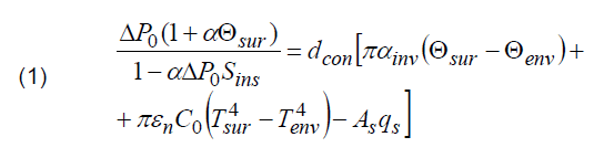
where ΔP₀ = I²r₀ is active power losses in the wire with linear resistance r₀. reduced to 0 ºC [kW/km]; I is current [A]; α is temperature coefficient of resistance [ºC^-1]; Θ_sur and Θ_env is the surface temperature of the wire and the environment temperature [ºC]; d_con is wire diameter [m]; S_ins is linear thermal insulation resistance [(ºC·m)/W]; α_inv is heat transfer coefficient by forced convection [W/(m²·К)]; ε_п is wire surface blackness ratio for infrared radiation; C₀ = 5,67·10-8 [W/(m²·K4)] is black body radiation constant; T_sur and T_env are absolute temperatures of the surface of the wire and the environment [K]; As is absorption capacity of the wire surface of solar radiation; q_s is solar radiation flux density on the wire [W/m²].

Equation (1) is written under the assumption that the temperature gradient in the conductor is zero. Then the temperature of the conductor wire is related to the temperature of its surface by a simple ratio:

where ΔP is active power losses, which is the left (and right) part of equation (1).

In equation (1), the losses in the left part are written as a function of the surface temperature of the wire (in order to eliminate the temperature of the core). It is easy to show that the relation:

is equivalent to a formula:

Bare wire can be considered as a special case when S_ins = 0. In the absence of isolation, the heat balance equation takes the form [5]:

The above formulas allow us to determine the temperature of the wire and the losses of active power taking into account the heating. The main drawback of this approach is that a large number of additional source data is needed: the parameters Θ_env, S_ins, α_inv, ε_п, A_s, q_s. The greatest problem is the heat transfer coefficient and solar radiation, which are determined by the whole set of meteorological conditions and vary not only in time but also along the route of each line (in particular, α_inv and q_s depend on the azimuth of the wire axis).

The main idea of the simplification of the task is the linearization of equations (1) and (5) as follows:

where R₀ is active resistance of the wire at 0 ºC [Ω]; A is the constant coefficient which determines the intensity of heat transfer from the wire to the environment.

Equation (6) is considered fair for both bare and insulated wires. Calculation per phase and per unit length in this case does not make sense anymore, therefore equation (6) is written for the three-phase line, and the resistance R₀ is reduced to the actual length. Thus, the left side of equation (6) represents the power loss in the entire line.

Having resolved (6) with respect to the temperature of the wire and substituting the result in the left side of the equation, we obtain the final formula for the losses in the line taking into account heating:

The numerator in this expression is the losses reduced to the environment temperature, and the denominator takes into account the increase in losses due to heating of the wires with a load current.

The coefficient A is determined by equation (6) at the maximum allowable current I_all:

where Θ_all is maximum wire temperature [ºC]; Θ_env1 is the temperature of the environment to which the maximum allowable current is reduced [ºC].

It can be seen that formulas (7) and (8) require a much smaller amount of source data compared to equations (1) and (5). Only the ambient temperature is required out of the entire set of meteorological parameters.

Comparative analysis

The results of comparison of the temperature of the wire and the power losses in the line, calculated by the simplified equations (6)-(8) and by the full models (1), (2), (5) are given below. The following objects were chosen as comparison objects:

bare wires of standard construction AS-240/32; high voltage insulated wires SIP-3 1×95 (analogue SAX); high temperature bare wires ACCR-405-T16.

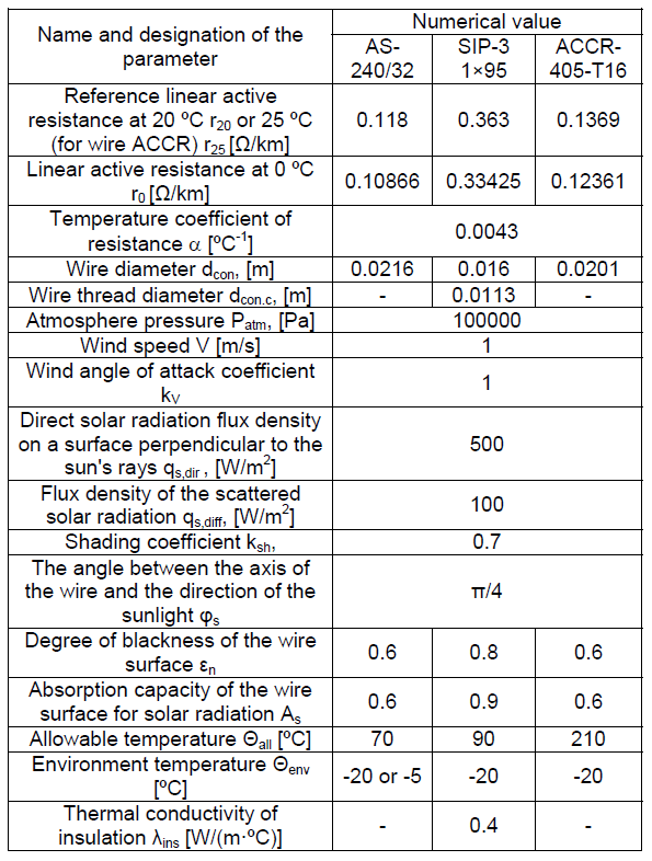
In all cases, a three-phase wiring system is considered. The parameters of the wires and cooling conditions are presented in Table 1.

The heat transfer coefficient, thermal insulation resistance and the flux density of solar radiation were determined by the following formulas [5], [6]:

The maximum value of direct solar radiation at the earth’s surface is about 1000 W/m². However, this value cannot be used to calculate energy losses, since direct solar radiation has an annual and daily rate, decreasing to zero at night. Therefore, the averaged value was used in the calculations, for which, in the first approximation, half the maximum was taken, that is q_s,dir = 500 W/m².

Table 1. Source data for calculations

Scattered radiation also has an annual and daily rate. The data allow to accept as a typical value q_s,diff = 100 W/m².

The shading coefficient k_sh shows how much of the total line length is, on average, illuminated by the sun during daytime hours. The value of k_sh = 0.7 is chosen taking into account the fact that the main part of the existing lines passes at sufficiently large distances from high structures. For lines of 110 kV and above, we should expect even higher values of the shading coefficient, since the supports have a greater height, and the main part of the lines passes in uninhabited areas. However, for 10 kV lines located near communications, the shadow coefficient may, on the contrary, be lower.

The angle between the axis of the wire and the direction of sunlight φ_s is assumed to be 45º as the average value between zero and 90º. In reality, it is determined by the average azimuth of the wire and the latitude of the terrain.

Tables 2-5 and Fig. 1-5 show the results of loss and temperature comparison for the wires under study. Tables 2-4 are built under the following conditions:

• environment temperature is minus 20 ºC;
• allowable currents are calculated on the basis of equations (1), (2) or (5) with the data presented in Table 1, but excluding solar radiation.

The low air temperature is chosen due to the fact that this corresponds to the expansion of the operating temperature range of the wires. As a result, the differences between exact and simplified methods become more pronounced.

The data in Table 5 were obtained with the reference value of the allowable current, taking into account the correction factor for the ambient temperature. The temperature of the environment is at a minimum level of -5 ºC, included in the table of correction factors.

Table 2. The results of the comparison of power losses and temperature of the wires AS-240/32 with the calculated allowable current

Table 3. The results of the comparison of power losses and temperature of the wires SIP-3 1 × 95 at the calculated allowable current

Table 4. The results of the comparison of power losses and temperature of the wires ACCR-405-T16 at the calculated allowable current

Table 5. The results of the comparison of power losses and temperature of the wires AS-240/32 at reference allowable current

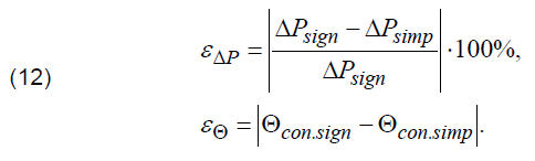
The load current I is expressed in fractions of the allowable current. The subscript “sign” for temperature and active power losses indicates the exact value calculated by equations (1), (2) and (5). The subscript “simp” corresponds to the simplified formulas (6) – (8). For the external temperature of the insulated wire, the additional index is not indicated, since the external temperature can only be calculated from the full model. Each Table also shows the relative errors in calculating the power losses ε_ΔP using the simplified formulas compared with the full formula (1), (2) or (5), and the absolute errors in calculating the temperature of the wire ε_Θ using the same methods:

It can be seen that the simplified formula gives the greatest accuracy for the wires AS-240/32 at the calculated allowable current. The dependences of power losses on the load current without solar radiation, constructed according to exact and simplified formulas, are practically the same on the scale of Figure 1. The calculating error for insulated wires slightly increases, but this increase is not significant. From a practical point of view, the error in calculating losses by simplified formulas becomes significant only for ACCR wires, where it can exceed 5%. The dependence of the calculating error on the type of wire is due to the increase in the operating temperature range: for the AS wires, with received data, it is 90 ºC, for SIP – 110 ºC, and for ACCR – 230 ºC.

The error in calculating power losses is conditionally systematic: the simplified method gives lower values of temperature and power losses compared to exact equations. However, a constant component of the error cannot be determined without taking into account solar radiation, since the error becomes zero at the allowable current and at zero.

Solar radiation at the accepted values of its intensity leads to additional heating of wires by 4-7ºC and to an increase in active power loss by about 2% (Tables 2-4). As a result, the difference between the exact and simplified methods increases with the appearance of the constant component of the error.

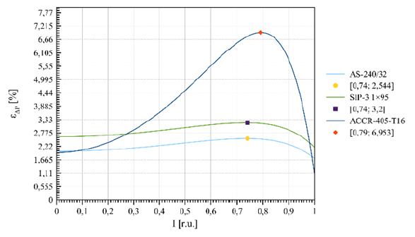
When using the calculated allowable current, the dependences of the calculating error on the load current have a clearly defined maximum both with and without solar radiation. The maximum points are highlighted in Fig. 4 and 5 with the abscissa and ordinate indicated. For all cases, the peaks are observed roughly in the same area – about 75-80% of the allowable current. At lower currents, the calculating errors are reduced due to the fact that the temperature of the wires decreases and the thermal change in resistance becomes less significant. The decrease in errors with increasing current over 80% of the allowable one is due to the fact that the coefficient A in the simplified formula is chosen from the condition of equality of the losses at the allowable current according to the exact and simplified methods. Therefore, with an allowable current, the error approximately corresponds to the constant component due to solar heating, and without solar radiation, this error is zero.

The considered laws are fully valid only for the case when the allowable current is calculated on the basis of the full heat balance equation. If the reference value of the allowable current is used in the calculations, which is not quite consistent with all the actual cooling conditions, the calculating error increases significantly when the simplified formula is used (Table 5, Fig. 3). Since the reference values of allowable currents are almost always less than the actual ones, the simplified formula in this case, on the contrary, gives overestimated values of the power losses. Corresponding errors may exceed 10%.

Conclusion

The results of the comparison of the accurate and simplified methods for calculating the active power losses in power lines taking into account the temperature allow us to draw the following conclusions:

1. In standard bare AS wires, as well as in insulated SIP-3 wires, the calculating error of losses by the simplified method does not exceed 3.2% compared to exact equations. The calculating error of losses in these wires becomes less than 1% in the absence of solar radiation.

2. Solar radiation increases the losses by about 2% regardless of the load. This should be considered the maximum estimate, since the conditions adopted in the calculations roughly correspond to the maximum possible average annual solar radiation. Consequently, this factor has almost no effect on the effectiveness of the measures to reduce energy losses and, therefore, in almost all cases can be excluded from the calculations.

3. In high-temperature wires, the calculating error may slightly exceed 5%; this is observed in the load range of about 70-90% of the allowable current.

These conclusions are valid for the stationary thermal regime and provided that the allowable current used in the simplified formulas fully corresponds to the exact equation of thermal balance. Reducing the accuracy with which the allowable current is set, leads to a significant increase in the calculating error of the losses (to about 10% in the AS wires).

The developed technique can be used for calculation and reduction of the energy losses in AS and SIP wires, as well as in most cases in wires of increased capacity. It allows taking into account the dependence of the resistance on temperature and at the same time avoiding the cumbersome calculations typical for solving the equations of thermal balance. The simplified formula for power losses has a clear physical meaning and requires only two additional data as compared to calculations without taking temperature into account: the allowable current and the environment temperature.

REFERENCES

[1] D. Douglass, “Weather-dependent versus static thermal line ratings [power overhead lines]”, Power Delivery IEEE Transactions on, vol. 3, no. 2, pp. 742-753, Apr. 1988.
[2] V.T. Morgan, “Effect of elevated temoerature operation on the tensile strengthof overhead conductors”, Power Delivery IEEE Transactions on, vol. 11, no. 1, pp. 345-352, Jan. 1996.
[3] S.L. Chen, W. Z. Black, H. W. Loard, “High-temperature ampacity model for overhead conductors”, Power Delivery IEEE Transactions on, vol. 17, no. 4, pp. 1136-1141, Oct. 2002.
[4] S.S. Girshin, A. A. Bubenchikov, T. V. Bubenchikova, V. N. Goryunov and D. S. Osipov, “Mathematical model of electric energy losses calculating in crosslinked four-wire polyethylene insulated (XLPE) aerial bundled cables,” 2016 ELEKTRO, Strbske Pleso, 2016, pp. 294-298. DOI: 10.1109/ELEKTRO.2016.7512084.
[5] H. Kocot, P. Kubek “The analysis of radial temperature gradient in bare stranded conductors,”Przegląd Elektrotechniczny, vol.10, pp. 132–135, 2017. DOI: 10.15199/48.2017.10.31.
[6] S.S., Girshin, A.A.Y, Bigun, E.V., Ivanova, E.V., Petrova, V.N., Goryunov, A.O., Shepelev The grid element temperature considering when selecting measures to reduce energy losses on the example of reactive power compensation // Przeglad Elektrotechniczny. 2018. No. 8. P. 101-104. DOI 10.15199/48.2018.08.24.
[7] J., Teh, I., Cotton Critical span identification model for dynamic thermal rating system placement // IET Generation, Transmission & Distribution. 2015. Vol. 9, Iss. 16, pp. 2644-2652. DOI: 10.1049/iet-gtd.2015.0601.
[8] Goryunov V.N., Girshin S.S., Kuznetsov E.A. [and etc.] A mathematical model of steady-state thermal regime of insulated overhead line conductors // EEEIC 2016 – International Conference on Environment and Electrical Engineering 16. 2016. С. 7555481.
[9] “Std 738”, Standard for calculating the current temperature of bare overhead conductors, 2006.
[10] “Thermal behaviour of overhead conductors”, Aug. 2002.

---

Authors: Stanislav S. Girshin, e-mail: stansg@mail.ru: Oleg V. Kropotin, e-mail: kropotin@mail.ru.; Vladislav M. Trotsenko, e-mail: troch_93@mail.ru; Aleksandr O. Shepelev, e-mail: alexshepelev93@gmail.com; Elena V. Petrova, e-mail: kpk@esppedu.ru; Vladimir N. Goryunov, e-mail: vladimirgoryunov2016@yandex.ru. Correspondence author e-mail: alexshepelev93@gmail.com

---

Source & Publisher Item Identifier: PRZEGLĄD ELEKTROTECHNICZNY, ISSN 0033-2097, R. 95 NR 7/2019. doi:10.15199/48.2019.07.10