Published by Janusz TYKOCKI1, Yong YUE2, Andrzej JORDAN3, The State College of Computer Science and Business Administration in Łomża (1), University of Bedfordshire (2), Visiting professor at University of Bedfordshire (UK), The State College of Computer Science and Business Administration in Łomża (3)
Abstract. The paper presents the distribution of temperature field in high voltage cables, 64/110 kV, (2XS (FL)) with copper conductor, depending on the depth of their arrangement in the soil and the soil thermal conductivity. Used to simulate the professional program NISA / Heat Transfer in the calculation using the finite element method (FEM).
Streszczenie. W pracy przedstawiono analizę rozkładu pola temperatury w kablach wysokiego napięcia 64/110 kV, (2XS(FL)) z żyłą miedzianą, w zależności od głębokości ich ułożenia w ziemi i wartości przewodności cieplnej gruntu. Do symulacji zastosowano profesjonalny program NISA/Heat Transfer wykorzystujący w obliczeniach metodę elementów skończonych (MES). (Analiza pola temperaturowego w układach kablowych 110 kV).
Keywords: thermal field, maximum temperature, 110 kV cables, FEM.
Słowa kluczowe: pole temperaturowe, temperatura dopuszczalna, kable 110 kV, MES.
Introduction
Overhead high voltage lines, which have been used to provide electrical energy supply, are currently often replaced by underground cable lines. The change is dictated by the requirements of spreading urbanization as well as by environmental needs: it is often necessary to transfer electric energy through the areas of national and natural landscape parks, watersheds, military areas, airports, etc.
The principal factor which limits the amount of energy possible to transfer by means of three-phase cable systems is temperature of the main conductor. The distribution of thermal field in underground cable systems is reliant on many determinants, among them being: distance from the surface of the ground, soil’s humidity and thermal conductivity, air temperature and wind velocity over the surface of the ground. Maximum temperature in the core of the cable should not exceed the allowed value given by the manufacturer (900 C in the case considered in this paper).
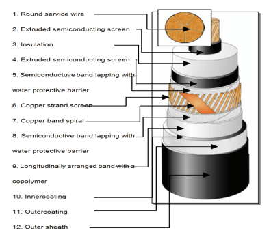
Structure of high voltage power cables
High voltage power cables are characterized by a special structure. The conductive core is shielded by protective insulation layers, and by a screening metal band grounded on one or both ends of the cable that, in certain cases, forms an additional source of heat, generating between 10% and 30% of the heat loss value in the main conductor. Figure 1 presents the exact structure of a high voltage power cable with copper conductor.
Cables using cross-linked polyethylene (XLPE) insulation were introduced in the beginning of the 1960s for the medium voltage range. Also, since 1971 the use of XLPE insulation has been widespread in 123 kV lines. Currently 500 kV cables are manufactured and successfully employed in the power industry.
The XLPE insulation is formed by a single-layer of uniform dielectric material made of cross-linked polyethylene (XLPE). The base material, i .e. polyethylene (PE), is a hydrocarbon having the form of a molecular chain which, due to its non-polar structure, exhibits excellent dielectric properties. The cross-linked structure is obtained through extrusion.
Over the compacted copper or aluminum strands, the inner conductive layer is placed. The layer is manufactured in a single technological process with the insulation and the external conductive layers covering it. The copper wire screen layer is produced by spreading over the waterproof coating that expands in a longitudinal direction and, in the case of potential sheath damages, prevents penetration of water into the inner layers. As for the outer sheath, it is made of anti-abrasive polyethylene. Overall, the cross-wise water-resistance of the cable is achieved by placing a coated aluminum band under the outer sheath, permanently conjoined with the polyethylene coating.
In approximately stable electrical and dielectric conditions, the increased heat resistance translates into the greater current carrying capacity in the full-time operation mode as well as in the case of short circuit.
• Lower loss factor tan δ = 4×10⁻⁴
• Relative permittivity εr = 2,4 (and as a consequence lower working capacity)
• Smaller weight
• Smaller bend radius
• Ease of handling during the arrangement
• Straightforward assembly of accessories
• No requirement for maintenance service.
Underground arrangement of cables
Running cable lines underground demands taking certain precautions against mechanical damages, rodents, or, in general, unintentional human actions that may occur during earthworks. That is why the cables are placed in concrete conduits filled with air.
In the following part the paper presents results of calculations concerning the distribution of thermal field in high voltage power cables, placed underground in different geometrical arrangements depending on soil’s thermal conductivity, distance from the surface of the ground, etc.
Climatic influences on the soil temperature
Distribution of temperatures within the earth’s crust is very diversified. The fundamental parameter characterizing thermal field of the Earth is geothermal gradient. It determines the temperature increase rate with the increasing unit of depth in the Earth’s interior, below neutral thermal zone. The inverse parameter geothermal degree specifies the number of meters into the Earth’s interior with which the temperature increases by 1oC [1], and its value is contained within a broad range. In particular, the most extreme values noted were in Budapest (15m/1oC) and in Republic of South Africa (144m/1oC). The value of geothermal gradient depends on such factors as the depth of igneous rocks deposits, thermal conductivity of rocks, tectonics, natural topography, volcanic, radioactive and geochemical activity, as well as certain hydro geologic processes.
Temperature distribution in the soil is a resultant of:
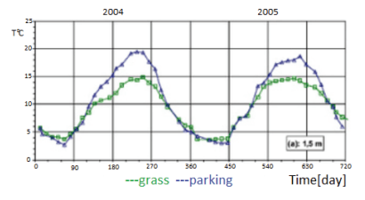
• Climatic influences depending on the climate zone, and weather influences (air temperature and humidity, solar radiation intensity, precipitation, wind) (fig.2).
• Ground surface type (e.g. bare ground with no vegetation, grass, concrete, snow layer).
• Structure and physical properties of the soil (density, permeability, thermal conductivity) (fig. 2).
Heat equation
Distribution of non-stationary thermal field for an underground cable can be described with the heat equation [3]
where: g(M)=j2ρ [W/m3] is the efficiency of spatial heat sources j [A/m2] is the current density in the core, ρ [Ωm] is the electrical resistivity of the wire (i .e. copper), λ [W/mK] is the thermal conductivity of the wire, insulation layers, and soil, whereas κ [m2/s] is the diffusion coefficient. Stationary thermal field T(x,y) of high voltage power cables placed underground, assuming a homogeneous and isotropic environment, in a two-dimensional system and specified conditions is described by the equation [3]:

This article discusses stationary thermal field T(x,y) of the system presented in figure 3, modeled by the equation (2). For the purpose of analysis of the stationary field, the following boundary conditions were assumed:

• On the lower horizontal line the temperature value of 8oC
• On the upper horizontal line the heat transfer conditions, where variables are wind velocity and temperature of air above the surface of the ground
• On the side lines the homogeneous second-type boundary condition.
Numerical model of the cable
The selection of suitable power cable, together with other relevant parameters, was based on technical specification provided by Tele-Fonika Kable S.A .:
• A2XS(FL)2Y2Y-GC-FR 1x2000RMS/210 64/110 (123)= kV IEC 60840
• Long-term current carrying capacity I = 940 A
• Maximum allowed core temperature: 90oC
• Heat conductivity of copper λcu = 360 W/mK (the following value is assumed in professional literature 395-401 W/mK)
• Heat conductivity of polyethylene λXLPE = 0,3 W/mK
• Electrical resistivity of copper ƍcu = 1,75×10⁻⁸ Ωm
• Heat conductivity of the soil in which the cables were placed: λz between 0,2 W/mK and 1,2 W/mK
• Convective heat transmission coefficient for the stagnant air over the surface of the ground ε = 16,6 W/m2K
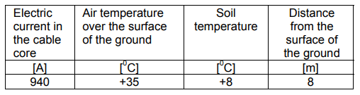
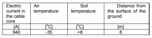
Tables 1-3 show the boundary conditions and air temperature, assumed in analysis of the cable systems.
Table 1. Boundary conditions
It must be pointed out that the boundary condition shown in Table 1 (+8oC) refers to the depth of 8 m contrary to the temperature of +20oC which occurs at the depth of 1.5m as presented in Figure 2.
Figure 3 presents the numerical model of the analyzed system for typical boundary conditions (table 1), assuming the heat conductivity of the soil λ = 1 W /m K.


Analysis of temperature distribution in the core, screen and on the surface of the cable for various distances from the surface of the ground and different values of soil’s heat conductivity
Figure 4 illustrates dependencies between the temperature of cable core and the heat conductivity of the soil. Considerable differences can be noted in the temperature of the core with the soil conductivity λz taking different values up to 0,8 W/mK.
Figure 5 considers thermal changes in the core (Tc), screen (Tsc), and on the surface of the cable (Tsr), with the constant heat conductivity of the soil λz equal 1,0 W /mK at variable depths from 1 m to 40 m under the surface of the ground. It can be seen that below 10 m underground the temperature of the core becomes stable (fig. 5).


Analysis of temperature distribution in the core of the cable for different air temperatures and with different distance from the surface of the ground
The results of the calculations for different boundary conditions are discussed above.
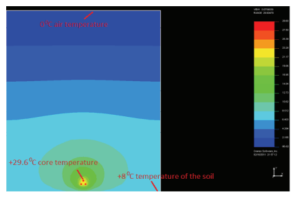
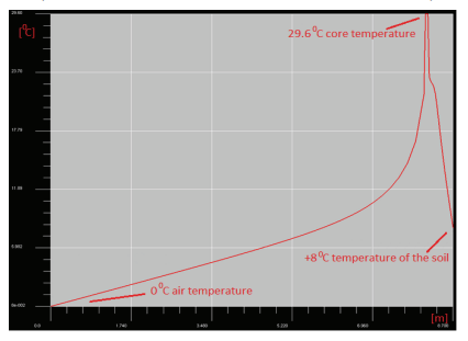


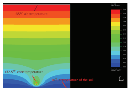
Moving to the temperature field distribution, figure 6 and figure 7 show the temperature in the analyzed system. In this case the core receives the highest value equal to 32.5oC. With these assumptions (table 2), the distribution of thermal field is illustrated in figure 8 and figure 9. In the discussed case, the temperature of the core dropped to 29,6oC.
The final result presented in Figures 10 and 11 shows the temperature in the main core equal to 27,3oC for the air temperature of -35oC.
Results concerning the investigation with the ground surface temperatures equal +35oC, 0oC, and -35oC, illustrating the dependence between the distance of the cable from the surface in the range of 1 m and 40 m and the temperature of the cable (preserving the other boundary conditions) are shown in figures 12-14.


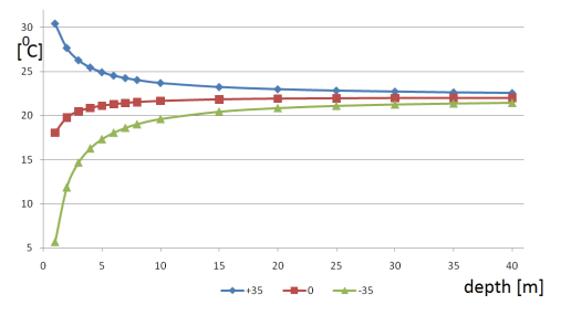
Table 2. The boundary conditions for air temperature 0oC
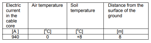
Table 3. The boundary conditions for air temperature -35oC
Conclusion
In the effect of the conducted computer simulation and the ensuing analysis of temperature distribution in the considered system depending on its distance from the surface of the ground and the heat conductivity of the soil the following conclusions can be drawn:
• heat conductivity of the soil has a significant impact on the temperature of the cable core – even up to the value of 0,8 W/mK
• temperature of the core stabilizes below the distance of 10 m underground
• thermal divergences between the core, screen, and the surface of the cable for given boundary conditions are constant and equal to 6oC and 2oC respectively, their values also stabilizes below 10 m underground
REFERENCES
[1] Geological Institute (in Polish) http://www.pgi.gov.pl/
[2] Heating systems (in Polish) http://systemyogrzewania.pl/
[3] Kącki E. Partial differential equations in problems WNT, 995
[4] Cranes Software, Inc http://www.nisasoftware.com
[5] Kacejko L., Karwat Cz., Wójcik H.: Laboratory techniques for high voltages (in Polish), WPL Lublin 2010
[6] Szpor S.: The technique of high voltages, WNT Warszawa 1967
[7] Flisowski Z.: The technique of high voltages, WNT 1998
[8] Gacek Z.: High-voltage isolation technology, WPS Gliwice 1996
[9] Khajavi M., Zenger W., Desing and commissioning of a 230 kV cross linked. Polyethylene insulated cable system, JICABLE 2003, Paris, paper A .1.1
[10] Toya A., Kobashi K., Okuyoma Y., Sakuma S., Higher stress desingned XLPE insulated cable in Japan, General Session CIGRE 2004, paper B1-111
[11] Suzuki A., Nakamura S., Tanaka H., Installation of the world’s first 500 kV XLPE cable with intermediate joints, Furukawa Review, (2000), n.19, 116-122
[12] Rakowska A., Recent advances in the field of high voltage cables. The use of copper wires in cables for voltages of 110 kV and higher, XII Scientific Conference – Technical power cable lines and outdoor Kable 2005 (in Polish), Zakopane paper 73-86
[13] Granadino R., Plans J., Schell F., Undergrounding the first 400 kV transmission line in Spain using 2500 mm2 XLPE cables, JICABLE (2003),Paris, A.1.2
[14] Jones S.L., Bucea G., Jinno A., 330 kV cable system for the MetroGrid project in Sydney Australia, CIGRE General Session (2004), paper B1-302
[15] Luton M., Anders G., Braun J-M., Downes J., Real time monitoring of power cables by fibre optic technologies tests , applications and outlook, JICABLE (2003), Paris A.16
[16] Royer C., Awad R., Boyer P.,Choquette M., Ferland P., Gignac R., Parapal J.L., A new generation of optimised 120 kV cable system at Hydro-Quebec JICABLE (2003), Paris, A.2.3
[17] Kobayashi S., Tanaka S., Suetsuhu M., Development of Factory Expanded Cold-Shrinkable Joint for EHV XLPE Cables, JICABLE (2003), Paris, A.5.1
[18] Mokański W., Mikołajczyk J., High voltage cable systems, XII Scientific Conference – Technical power cable lines and outdoor Kable 2005 (in Polish), Zakopane paper 105-112
[19] Rakowska A., Cable or aerial line – not just a technical dilemma, II National Conference on Electricity in rural areas, (in Polish) ETW 2004 Jachranka 2004, paper 59-70
[20] Rakowska A., Criteria for verifying the quality of cross-linked polyethylene insulation for use as power cables, Poznań (2000)
[21] Beghin V., Geerts G., Liemans D., Double 150 kV link, 32 km long, in Belgium: design and construction, CIGRE Session 2004 B1-305
Autorzy: Janusz Tykocki, The State College of Computer Science and Business Administration in Łomża, http://www.pwsip.edu.pl, ul. Akademicka 14, 18-400 Łomża, E-mail: jtykocki@pwsip.edu.pl Yog Yue, University of Bedfordshire, e-mail: Yong.Yue@beds.ac.uk Andrzej Jordan, Visiting professor at University of Bedfordshire(UK) The State College of Computer Science and Business Administration in Łomża, http://www.pwsip.edu.pl, ul. Akademicka 14, 18-400 Łomża, E-mail: ajordan@pwsip.edu.pl
Source & Publisher Item Identifier: PRZEGLĄD ELEKTROTECHNICZNY (Electrical Review), ISSN 0033-2097, R. 88 NR 6/2012.
