Published by Patrick S. Pouabe Eboule, & Ali N. Hasan, University of Johannesburg, South Africa
Abstract. In this paper a new approach for the detecting and locating different kinds of faults on power transmission lines using the concurrent neurofuzzy technique (CNF) is introduced. This approach relies on the advantages of combining fuzzy logic (FL) and the artificial neural network (ANN) to detect, classify and locate faults on a power transmission line that carries high voltage and very high voltage of 400 kV and 750 kV respectively over short distance and long distance of 120 km and 600 km respectively. Results exhibit that CNF is capable of detecting several and different fault types and locations with high accuracy, which will reduce the time for the technical team maintenance to achieve their goals.
Streszczenie. Wartykule przedstawiono nowe podej´scie do wykrywania i lokalizowania ró˙znego rodzaju usterek w liniach elektroenergetycznych przy u˙zyciu współbie˙znej techniki neuro-rozmytej (CNF). Podejs´cie to opiera sie˛ na zaletach poła˛czenia logiki rozmytej i sztucznej sieci neuronowej w celu wykrywania, klasyfikowania i lokalizowania usterek w linii elektroenergetycznej, która przenosi wysokie napi˛ecie i bardzo wysokie napi˛ecie odpowiednio 400 kV i 750 kV w krótkim czasie odległos´c´ i długa odległos´c´ odpowiednio 120 km i 600 km. Wyniki pokazuja˛, z˙e CNF jest w stanie wykryc´ kilka róz˙nych typów usterek i lokalizacji z duz˙a˛ dokładnos´cia˛, co skróci czas potrzebny zespołowi technicznemu na osia˛gnie˛cie celów. (Precyzyjne wykrywanie i lokalizowanie usterek w linii przesyłowej energii przy u˙zyciu równoległej techniki neuro-rozmytej)
Keywords: Transmission Line Systems, Fault Detection, Fault Location, Concurrent Neuro-Fuzzy Technique
Słowa kluczowe: Systemy linii przesyłowych, Wykrywanie uszkodze´ n, Lokalizacja usterki, Równoczesna technika neuro-rozmyta
Introduction
The first AC power transmission line system was initially introduced in the year 1889 in the United States of America [1]. The first electrical transmission line was connected between Oregon city and Portland. This line was characterized by a line voltage of 4 kV, single phase with a length of 21 km. However, the first three-phase system was introduced and built in Germany in 1891. The transmission line covered a distance of 179 km at 12 kV[1].
AC power transmission line systems have been researched and improved since it was first introduced. Powerful transmission line systems have been implemented and installed all over the world to meet the ever growing energy demand over the years. Nowadays, we are able to transmit electrical energy at various distances using modern and sophisticated power transmission systems. However, these sophisticated energy transmission systems come with limitations and challenges. Therefore, there is need to continuously monitored and maintained the power transmission lines in order to eliminate catastrophic breakdown and disruption of services to the end user costumers[2, 3, 4].
Several techniques and approaches have been developed by various researchers for troubleshooting and detecting faults in transmission power lines. These techniques include discrete Walsh-Hadamard transform, discrete wavelet transform, naive bayes classifier, hilbert huang transform and k-means data description method. However, these techniques come with limitations and did not perform optimally when applied for detecting and locating faults.[5, 6, 7, 8, 9, 10].
In 2020, Aker et al. used wavelet transform and naive bayes classifier to identify the type of fault that may occur in the shunt compensated static synchronous compensator. The network was designed using Simulink and faults were applied at disparate zones. The technique decomposed the obtained waveforms into several levels using Daubechies mother wavelet and applied naive bayes to classify the faults. It emerged from this study that the accuracy could be up to 80%. However, only fault classification was implemented [5].
Earlier in 2019, Kapoor applied a discrete Walsh- Hadamard transform to detect faults and identified faulty phase in a three phase transmission line connected with distributed generation. In this technique, the fault data was recorded using characteristics based on Walsh-Hadamard coefficients of the current. It emerged from this research that the method can effectively identify the fault phase [8, 9]. The same year, Hosein et al. proposed and applied ANFIS technique for detecting faults in smart grids. The currents measured at only one side of a three-phase transmission line is collected and passed through a signal processing module. The results obtained are compared against other AI techniques (ANN and SVR). It emerged from this study that the best accuracy obtained is 87.5% for ANFIS technique which outperforms SVR and ANN techniques. However, this paper only dealt with faults location and did not propose faults classification. Moreover, only four different fault types were considered in obtaining the total dataset. The total accuracy obtained could have been improved on this case studied by increasing the size of the dataset [11].
As the transmission line grid continuously grows with the increasing demand on energy, it becomes more complex and difficult to prevent faults from occurring. Therefore, the convectional methods of troubleshooting and detecting faults in transmission lines are becoming inefficient and obsolete. Thus, the need to develop and implement new techniques that can accelerate the process of fault detecting and also ensure a good compatibility of the modern and complex electrical system is necessary [12]. In addition, the current methods of fault detection also suffer from a reliability problem because faults on transmission lines are often non-linear that is to say, there is no formal causal effect relationship between the detected fault and its origin. Therefore, these methods are unable to solve non-linear problems [13].
As a result, it was essential to develop an intelligent system that can predict, detect and locate different fault types. These fault detection systems use artificial intelligence techniques.
Power transmission lines are subject to multiple defects [14, 12, 15]. These faults and defects can be subdivided into different types of faults such as single line to ground fault (SLG), double line to ground fault (DLG), triple line fault (TL) and triple line to ground fault (TLG) [14, 12, 15, 16]. The most frequent fault that occurs on power transmission lines is the over-voltage fault, which comes from capricious atmospheric conditions such as lightning, bush fires and cyclones [17, 18]. These faults have a damaging and hazardous impact on the transmission lines and the power system in general [17].
Artificial Intelligence (AI) fault detection techniques have shown to be more accurate and more promising [19, 20, 21, 22]. Researchers have found a more robust approach and solution in solving complex problems by using different combinations of these AI techniques [23, 24]. In power transmission lines, fault types are numerous and diverse. Thus, faults are distinguished based on the meteorological conditions from those of an electrical/mechanical origin, coming from the production system [16].
Climate change is one of the causes of faults on power transmission lines. It can affect a cable by accelerating its ageing process [17, 18]. The use of AI techniques could accelerate the process of detection, classification and location of the faults over long power transmission lines carrying high voltage electricity. A Concurrent Neuro-Fuzzy method was used in this experiment because it combines two powerful AI techniques of fuzzy logic (FL) and neural networks (ANN). These two methods, FL and ANN, have repeatedly and successfully been used in different fields of engineering to solve problems where the traditional and classical methods have not been able to provide genuine solutions [19, 23].
In 2018, Eboule et al. proposed a fault detection and location algorithm based on concurrent neuro fuzzy. The technique consisted of setting various FL conditions and of using ANN to process them in order to detect, classify and locate 11 fault types that may occur in transmission lines. It emerged from this study that the accuracy of an AI system is directly linked to the number of data sets and the architecture of the system [2, 4]. However, this paper only dealt with one type of transmission line and did not take all significant transmission line’s parameters into consideration.
In 2015, Anamika et al. improved the performance of a transmission line using a fuzzy inference system. The method consisted of designing three distinct systems respectively for transmission line directional relaying, fault classification and fault location schemes using fault current and voltage available at the relay location. It emerged from this study that the proposed method can efficiently detect faults for both forward and reverse directions [25].
In 2013, Marjan et al. [26] implemented a fault location algorithm that can be used to locate various faults along mixed line-cable transmission corridors based on the telegraph’s equations. It emerged from this study that the use of Clarke transformation is powerful when dealing with transient studies. In 2012, Carlo et al. in [3] used FL to classify various faults in single and double circuit lines. They concluded that to improve the yield of their system, FL membership functions have been chosen to have an overlap with each other. A modified technique was proposed to increase the accuracy and the performance of the proposed FL fault detection in double-circuit was tested using 3000 cases. Early in 2005 Mahmoud et al. studied in [27] a combined overhead line with underground cable for fault location. The simulation was done via Matlab and it emerged from this implementation that the maximum error in the overhead section was 0.21% over 100 km while underground the error was 1.643% over 10 km.
The limitation found in the above literature is that CNF is not widely used in various engineering fields. However, Eboule in [2, 4] introduced the use of the CNF technique for power transmission line faults detection and location in a limited scale. This paper provides in depth use of CNF technique for power transmission line fault detection and location taking into consideration all significant parameters of the transmission lines and with a bigger data set and information used in two experiments. The obtained results are compared to [2] paper results and [4] paper results.
The main objective of this work is to introduce and use the powerful artificial intelligence technique called CNF technique for the application of power transmission line fault detection and location. This will be achieved by following a well-defined and structured sequential methodological approach of CNF functions in detecting and locating faults for two distinct power transmission lines. Comparison analysis with the previous studies will also be investigated to determine the performance efficiency of the proposed CNF technique. The first transmission line is characterized by its voltage of 750 kV over 600 km distance while the second transmission line has 400 kV over 120 km distance. The impact of this study could lead to reduced power system and transmission line maintenance cost and time. This will result in sustainable power delivery to customers and increased grid reliability. This will increase the income of the company supplier and will help developing a great business environment which is necessary to absorb the level of unemployed.
This article put forward four main contributions. The first contribution is the implementation of a new technique (CNF) to detect, classify and locate power transmission line faults for high voltage and very high voltage over short and long line lengths. The second contribution is the application of such a technique into a system that includes 11 different fault types and take all significant power transmission line parameters into consideration and compare the obtained experimental results. Knowing that this concurrent neuro fuzzy technique has been applied in [23] on surface roughness modelling in drilling. The third contribution is to investigate if this AI technique could be effectively applied for fault detecting and locating for long transmission lines. Because the application of the technique in transmission line is still new, thus, the fourth contribution is to demonstrate the robustness of the technique and to make it be common.
This paper is organized as follows. Section 2 introduces the CNF technique, Section 3 describes the experiment setup, Section 4 discusses the experimental results obtained and Section 5 presents the conclusions.
Concurrent neuro fuzzy technique
In these experiments a methodology using CNF that deals with two tasks of detecting and locating faults on PTLs is introduced. Two different data sets were used for the two tasks of locating and identifying the faults. Therefore the CNF was trained separately twice with each data set.
The concurrent neuro-fuzzy (CNF) technique was introduced by Jang Lin and Lee in 1991. Since then, the CNF technique has been successfully applied in many fields and tasks such as control tasks, data analysis, detection and classification. The CNF technique generally represents a set of two distinct FL and ANN methods used to solve a precise problem where the FL method determines the rules and ANN adjusts these rules [23]. FL has been used in many applications. It has been successfully used in exploiting and processing the data in different areas such as image processing, image recognition in medicine and video surveillance. It has become apparent that the greatest challenges of this method is the determination of the rules and the search for the appropriate membership function to reduce the percentage of error [24, 28, 29]. This allowed for the introduction of the ANN technique in data processing to make the algorithm more efficient in the assigned task. CNF allows FL and ANN to analyze the data together and concurrently. Figure 1. presents the general architecture of the CNF network.
In Layer 1, the obtained data from the post faults are directly transmitted to the next layer.


where yi(1) represents the output of all neurons in Layer 1 and xi(1) represents the input of Layer 1. In Layer 2, the fuzzification is applied. The membership function which was used is triangular sets and the two parameters, a and b, are determined as follows.

Where yi(2) is the output Layer 2, xi(2) is the input Layer 2 which is the X-axis in Figure 2 and a, b are parameters as follows in Figure 2.

In Layer 3, different fuzzy rules are defined. Intersection was implemented by the product operator as shown in Equation 2.

Where: yi(3) is the outputs of Layer 3 and xki(3) is the input of the (k) neuron in Layer 3. In Layer 4, the consequence of FL rules is represented. CNF uses the probabilistic OR operation to determine the outputs of each neuron.

Where: yi(4) represents outputs of Layer 4 and xki(4) is the inputs of the (k) neuron in Layer 4. In Layer 5, a single output of the neuro-fuzzy system was represented; it is the layer where defuzzification takes place. Output is computed by applying the sum product composite technique. Equation 4 presents how to compute the predicted output of the CNF network [23].
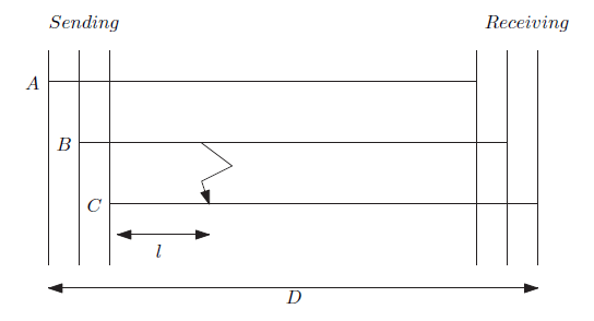
Table 1. Power transmission line parameters.
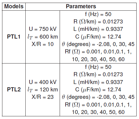

where, y represents the output of the neuro-fuzzy system and μck is (k) output of the layer 4.
Experiment setup
The experiment was conducted on a three-phase power transmission line (PTL) as shown in Figure 3 using the line parameters in Table 1 of the South African main energy supplier (ESKOM Ltd). These PTLs have the same R, L, C parameters but, the line voltage and the length of the lines are different. The experiment was simulated using MATLAB/ SIMULINK. All 11 faults were set manually using a logical signal to control the fault operation as shown in Figure 4. the ground and the fault resistances were defined. The sampling frequency for the fault simulator was set at 0.2 to generate each fault sample data. A 2200 data sample (11 faults × 10 fault resistances × 5 zones × 4 fault angles) were generated and collected from the post-faults (short-circuit voltage and current) and used for training and testing the CNF network. This sampling frequency corresponds to the rate at which the system samples its inputs.
At different distance along the line, different fault types were simulated in terms of fault angles and fault resistances in order to have all different types of faults with their location where they occurred on the PTL. The short-circuit voltage and current were recorded at the beginning of the line and used as the inputs for the experiments.

Four experiments were conducted, the split percentages for the two data sets of the fault type and the fault location was 70% to train and 30% to test. The experiments were conducted using successively 550, 1100 and 2200 data as mentioned in Table 3. The first two experiments were for fault type detection for long and short transmission lines whereas the third and the fourth experiments were for fault location for long and short transmission lines.
For the fault detection experiment, the CNF network shown in Figure 1 with 5 hidden layers were used. In these experiments, the structure of the CNF method was determined using the standardized data of the post faults. The computation number of neurons for each layer in the CNF network follows a certain number of rules such as the number of the inputs, the number of the FL conditions and the membership function type [2, 30, 33]. Thus, the determination of the most accurate CNF network structure for power transmission line fault type detection is obtained.
For Layer 1, six neurons were used, these neurons correspond to the required six input variables Va, Vb, Vc, Ia, Ib, Ic respectively. The six input variables represent the root mean square (RMS) of the short circuit voltage phase to ground and the short circuit current across the conductors A, B and C of the power transmission line. Data were normalized using the following normalization equation.

Where: Xn is the normalized data for each variable, Xmin, and Xmax are the minimum and the maximum values respectively.
In Layer 1, the output dimension represents the six input variables times the number of faults (6×2200). In Layer 2, three conditions have been established for the CNF algorithm so that the determination of the number of neurons at this layer corresponds to the number of conditions of the FL multiplied by the number of inputs data [31, 32]. The number of neurons for Layer 2 is 6×3 = 18 neurons. The output dimension obtained was the number of neuron times the number of faults (18×2200).
The three required FL conditions are N1,N2 and N3.

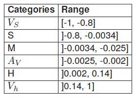
Table 2. Different ranges of the membership function
These conditions were determined as follow:

Pn parameters was found as follows:

where:

Ia, Ib and Ic are the post fault currents flowing in the A, B and C conductors of the transmission lines. The choice applied in Layer 2 was made according to the membership function of the data. For this experiment, a triangular membership function was used as shown in Figure 5, as soon as the the membership function categories with their values range obtained shown in Table 2.
Where: Very Small (VS), Small (S), Medium (M), Average (AV), High (H), Very High (Vh)
In Layer 3, each neuron corresponds to each fault type. Consequently, eleven neurons were necessary for 11 FL conditions [33]. The output dimension for this layer was obtained according to the number of FL conditions multiplied by the total number of data used (11 × 2200). In Layer 4, the number of membership functions is six which corresponds to the number of neurons.
Consequently, six neurons were necessary. The outputs of each neuron in this layer were determined by following the probabilistic OR approach and the dimension of the output in this layer is 6× 2200. In layer 5, the sum average of centroids technique was used to determine the output for the CNF network. It can be seen from Equation 8 that only current data were used to define and set the fuzzification rules. Usually one parameter is used in such experiment to set the FL rules in order to reduce the experiment computation time and complexity but the increasing of the input variables could reduced the obtained error [2]. The final output dimension obtained for fault classification is 1×2200. The different FL conditions used to set the CNF technique parameters are given below
• If N1 is Vh and N2 is H and N3 is VS then SLAG
• If N1 is VS and N2 is Vh and N3 is H then SLBG
• If N1 is H and N2 is VS and N3 is Vh then SLCG
• If N1 is VS and N2 is Vh and N3 is M then DLAB


• If N1 is VS and N2 is H and N3 is Vh then DLBC
• If N1 is Vh and N2 is VS and N3 is S then DLAC
• If N1 is VS and N2 is Vh and N3 is AV then DLABG
• If N1 is VS and N2 is S and N3 is Vh then DLBCG
• If N1 is Vh and N2 is S and N3 is S then DLACG
• If N1 is S and N2 is S and N3 is H then TLABC
• If N1 is S and N2 is S and N3 is Vh then TLABCG
Two experiments (experiment 1 and experiment 2) were carried out using CNF network for two transmission lines fault type detection. Experiment 1 and 2 algorithm is shown in Figure 6 flow chart. The algorithm steps are explained as follows:
• Load the file data
• Extract the input data from the data file
• If the Extraction is successful, normalize the input data, else repeat the previous step
• Define the output data
• Normalize the output data
• Define the functionality of each neuron in all layers from layer 1 to layer 5
• If the previous step is successful, initialize weights, else repeat the previous step
• Determine error in each neuron
• Update weights between different neurons
• Define the number of epochs
• Train and Test the concurrent neuro-fuzzy structure
For experiments 3 and 4, the structure of CNF for faults location in both lines is shown in Figure 7.
In these experiments, telegrapher’s equation was used to locate faults over power transmission lines. Telegrapher’s equation converts three phase lines to Clarke’s transformation to determine 0, alpha (α), and beta (β) variables [2, 34]. The utilization of Clarke’s transformation is recurrent in fault location because in PTL we have symmetrical and unsymmetrical faults. Three phase power transmission lines are presented in Figure 3 with a fault which occurs at l distance from the generation side.
The voltages and currents for the three phase transmission lines are transformed using Clarke’s transformation as the following:

and

Thus, fault distance parameters can be computed as:

where i = 0, α, β
lα and lβ are the two areal modes, l0 is the ground mode. γi, Zci, Υi and Zi are determined using the line parameters as shown in equation 12:

R, L, G and C are the lines parameters, the resistance, the inductance, the conductance and the capacitance respectively. Ai and Bi are determined using the line voltages, the line distance and the line impedance as shown in equations 13 and 14

and

An accurate fault location point can be determined by the appropriate mode 0, alpha, and beta. VS is voltage sending, VR is voltage received, D is total length of the line,

lα is valid for all types of fault except line to line faults where the lβ is applied.
The outputs from Layer 1 to Layer 5 have a 2200×6 dimension. However, after the data were split into 0, α and β variables respectively, the dimension outputs obtained in layer 5 were 600×1, 600×1 and 1000×1. The CNF algorithm for fault location is programmed by using Matlab software. Flow chart of the CNF algorithm for faults location is illustrated in Figure 8 and the proposed algorithm works as follows:
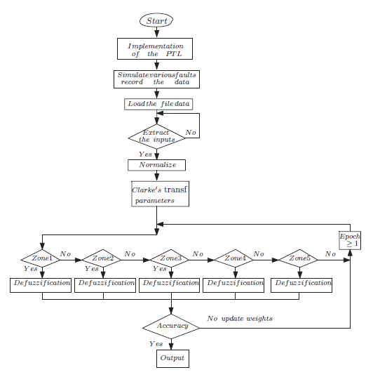
• Load data
• Define variable
• Layer 1 normalise input data and forward to Layer 2
• Layer 2 divide data to 0, α and β data
• Layer 3 apply Clarke’s transformation
• Layer 4 determine parameters transmitted (voltage and current)
• Layer 5 determine output distances
• Initialise weights, Determine error in each neuron
• Update weight in different neurons for each layer
• Define the number of epochs, Train and Test the system
Most important in error calculation is magnitude [35, 36, 37]. Thus values of error were determined for fault location using equation 16 .

where Ddesired represents the fault distance desired, Dpredicted the fault distance is determined using the algorithm and D the total length of the line.
Experiment Results and Discussion
Experimental results show that the best and most accurate results are obtained when using the 2200 data set as shown in Table 3. For this fault classification experiment, the number of neurons that characterize the topology of the CNF structure was determined according to FL rules. Thus, the structure of the CNF algorithm for the detection and classification of faults was the same for both transmission line short and long length which is 6-18-11-6-1.
The evaluation error was obtained by summing the various input data which do not satisfy the conditions established by FL and dividing this sum by the total number of data inputs. Therefore, the total achieved fault type prediction accuracy is approximately 97.5% for the long line and 95.6% for the short line.
Table 3. Fault location prediction results.
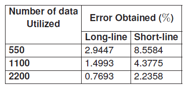
Table 4. CNF fault defuzzication output and FL conditions for the long line at 600 km, Rf = 0.001 Ω, fault angle = -2.0892 ◦ for the different fault types
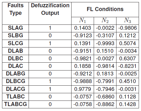
Table 5. CNF fault defuzzication output and FL conditions for the long line at 48 km, Rf = 0.001Ω, fault angle = -2.0892◦ for the different fault types

Table 4 and Table 5 respectively present the long and the short transmission line different fault types, as well as the defuzzification outputs obtained after FL conditions were applied. The obtained defuzzification output for DLAB, DLAC, TLABC and TLABCG are found to be approximately Zero. All the input variables which do not satisfy the conditions of FL were considered “Non-Applicable”fault conditions (N/A). The N/A input variables were used to determine the prediction accuracy error.
Figure 9 presents the sum of area of all faults which occurs at 600 km, Rf = 0.001 Ω and fault angle of -2.08920 without defuzzification for the long line and Figure 10 presents the sum of area of all faults which occurs at 120 km, Rf = 0.001 Ω and fault angle of -2.08920 without defuzzification for the short line.
Figures 9 and 10 are unique for each area where faults may have occurred and could be used to predict either fault classification or fault location. In [2] and [4], the authors demonstrated that the obtained defuzzification output which was tested at 120 km with Rf = 10Ω and a fault angle of 45 degrees shown in Figures 11 and 12 can also be used in order to classify and locate the exact faults that may have occurred in a very high voltage transmission line.
For faults location results, the CNF network structure was considered based on the different parameters obtained by Clarke’s transformation approach.
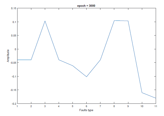
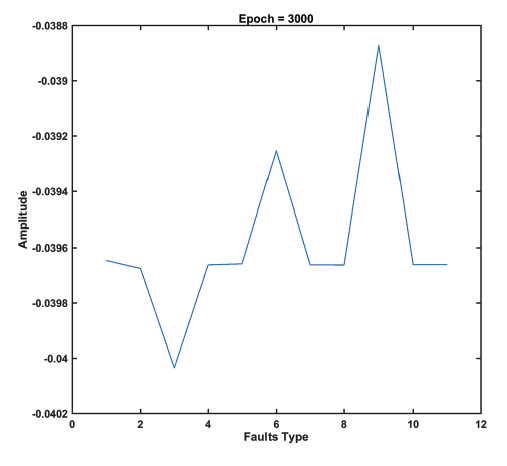
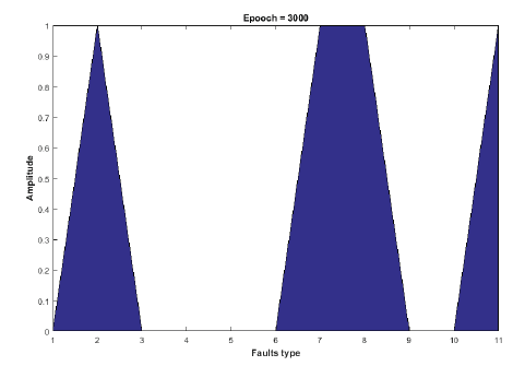
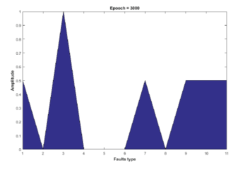
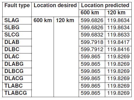
Table 6. Desired and Predicted fault location for the Long Transmission Line with Rf = 0.001Ω, fault angle = -2.0892◦
However, each parameter has been assigned single neuron thus, the structure of the CNF algorithm for the location of the faults was 6-6-6-6-3. The total achieved prediction accuracy for the long line is approximately 99.2309% for fault location and 97.77% for the short line. Table 3 presents various error obtained in respect of a range of data used in simulation.
Table 6 and Table 7 show the long and the short line fault type with its location predicted either at 600 km or at 120 km for the long transmission line and at 120 km and 48 km for the short line. Table 8 and Table 9 illustrate the fault location prediction errors for different locations for long and short transmission lines respectively with fault resistance of 0.001Ω and fault angle of -2.0892 degrees.
Table 7. Desired and Predicted fault location for the short Transmission with Rf = 0.001Ω, fault angle = -2.0892◦
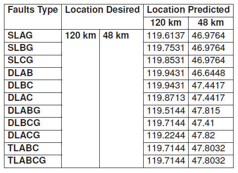
Table 8. Fault location errors for the long transmission line with Rf = 0.001Ω, fault angle = -2.0892◦
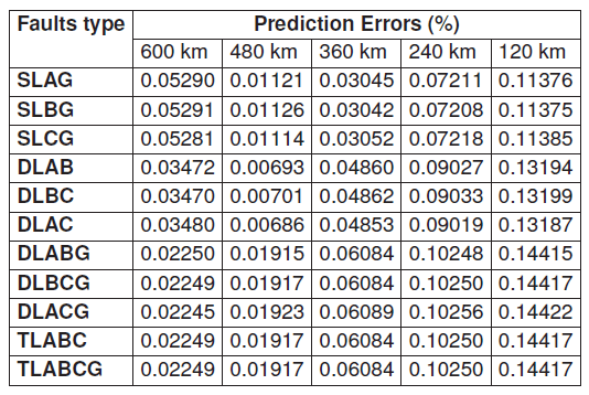
Table 9. Fault location errors for the short transmission line with Rf = 0.001Ω, fault angle = -2.0892◦
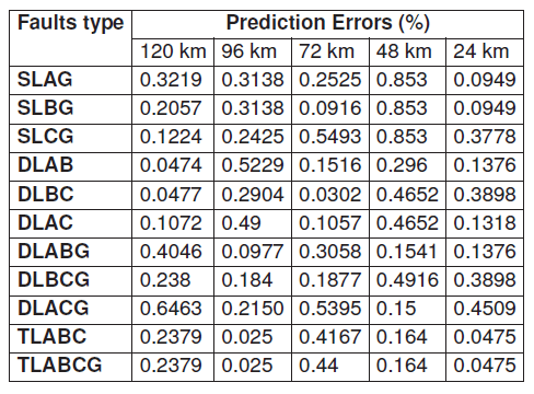
The fault locations errors were determined using equation 16. Comparing these two tables, it can be seen that at 120 km distance in Table 8, the obtained prediction errors are less than the 120 km distance in Table 9. This could be because of the nature of the utilized dataset.
The worst case scenario is likely to happen at any time if one of the fuzzy rules is not respected. For fault classification according to Table 5, the worst case is SLCG, appeared at 48 km with Rf = 0.001 ohm, fault angle = -2.0892 degree. This problem may occur for some reasons such as, the human error, the error on your data or/and on the algorithms.
In overall, the fault location algorithm for these two cases is more accurate for the long transmission line. However, The study results and findings clearly show that the proposed methodology to evaluate the system error is reliable and can achieve high accuracy which also support the results found in the previous studies published in [2] and [4].
Conclusion
In this article a novelty technique capable of detecting and locating faults in power transmission lines using the state of the art concurrent fuzzy neural network was developed. This technique was applied on two distinct power transmission lines that carry 750 kV over a length of 600 km for the long line and 400 kV over a 120 km length for the short line.
The challenge of applying this technique is to get a sufficient amount of dataset and defining FL rules. Thus, the experiment were carried out using Matlab/Simulink. Post-faults current and voltage were simulated and the obtained values were used as the data set. The proposed fault detection system algorithm for CNF was designed and tested using several faults data sets. Results showed that for both the fault classification and the fault location experiments, the CNF proposed technique achieve high accuracy for both long and short lines. However, the highest prediction accuracy of 97.5% for fault type detection and 99.2309% for fault location from the long line case study was obtained. This can be explained by the fact that the same FL conditions were applied on both systems and these conditions where determined using only the post-faults data from the long line. Thus, the experimental classification results could be improved by acting on the established conditions such as assigning separate rules to each power transmission line.
A comparison was made with other studies which investigate similar cases using CNF technique for fault classification and fault location was introduced. The results and findings of this experiment supports the findings for the other studies that CNF could be reliable and would perform well for the application of fault type classification and location on power transmission lines. It was shown that the defuzzification output can be used to classify various fault types and to locate them.
Finally, it can be concluded that the CNF could be used for fault prediction over three phase power transmission lines. Predicting fault location and fault type with high accuracy could minimize the maintenance cost and time. This will increase the power transmission process efficiency and reliability. CNF technique can also be tested on even longer transmission lines than the 600 km length studied, medium lines and even on multiphase power transmission lines such as six-phase system. Moreover, the effect of including CT could be investigated in future studies in order to determine the influence of using CT on the classification accuracy and the experimental results.
This CNF technique could be applied in various engineering fields following the procedure provided. The choice of parameters or inputs variables depend on the expert and will influence the results obtained.
REFERENCES
[1] Glover, J.D., Sarma, M.S. and Overbye, T., 2012. Power system analysis & design, SI version. Cengage Learning.
[2] Eboule, P.S.P., Pretorius, J.H.C., Mbuli, N. and Leke, C., 2018, October. Fault Detection and Location in Power Transmission Line Using Concurrent Neuro Fuzzy Technique. In 2018 IEEE Electrical Power and Energy Conference (EPEC) (pp. 1-6). IEEE.
[3] Cecati, Carlo and Kaveh Razi, (2012), Fuzzy-logic-based high accurate fault classification of single and double-circuit power transmission lines. In International Symposium on Power Electronics, Electrical Drives, Automation and Motion, pp. 883-889. IEEE.
[4] Eboule, P.S.P., Pretorius, J.H.C. and Mbuli, N., 2018, November. Artificial Neural Network Techniques apply for Fault detecting and Locating in Overhead Power Transmission Line. In 2018 Australasian Universities Power Engineering Conference (AUPEC) (pp. 1-6). IEEE.
[5] Aker, E., Othman, M.L., Veerasamy, V., Aris, I.B., Wahab, N.I.A. and Hizam, H., 2020. Fault Detection and Classification of Shunt Compensated Transmission Line Using Discrete Wavelet Transform and Naive Bayes Classifier. Energies, 13(1), p.243.
[6] Bachmatiuk A, I˙zykowski J. Distance protection performance under inter-circuit faults on double-circuit transmission line. Przeglad Elektrotechniczny. 2013;89(1):7-11.
[7] Dong AH, Geng X, Yang Y, Su Y, Li M. Overhead line fault section positioning system based on wireless sensor network. Przegla˛d Elektrotechniczny. 2013;89(3b):60-1.
[8] Kapoor, G., 2019. Detection and classification of four phase to ground faults in a 138 kV six phase transmission line using Hilbert Huang transform. International Journal of Engineering, Science and Technology, 11(4), pp.10-22.
[9] Kapoor, G., 2019. Protection technique for series capacitor compensated three phase transmission line connected with distributed generation using discrete Walsh-Hadamard transform. International Journal of Engineering, Science and Technology, 11(3), pp.1-10.
[10] Farshad, M., 2019. Detection and classification of internal faults in bipolar HVDC transmission lines based on K-means data description method. International Journal of Electrical Power & Energy Systems, 104, pp.615-625.
[11] Hassani, H., Razavi?Far, R. and Saif, M., 2019, October. Locating Faults in Smart Grids Using Neuro?Fuzzy Networks. In 2019 IEEE International Conference on Systems, Man and Cybernetics (SMC) (pp. 3281-3286). IEEE.
[12] Pouabe Eboule, P.S., Hasan Ali, N., Bhekisipho Twala, (2018) The use of multilayers perceptron to classify and locate power transmission line faults. In Artificial Intelligence and Evolutionary Computations in Engineering Systems, pp.51-58. Springer, Singapor.
[13] Pasupathi Nath R. and Nishanth Balaji V., (2014), Artificial Intelligence in Power Systems. IOSR Journal of Computer Engineering, p.2278-0661.
[14] De Metz-Noblat,B., Dumas, F. and Poulain, C., (2005) Cahier technique n 158 : Calcul des courants de court-circuit, Schneider Electric Collection technique.
[15] Hasan Ali, N., Pouabe Eboule, P.S., Twala B, (2017), The use of machine learning techniques to classify power transmission line fault types and locations. International Conference on Optimization of Electrical and Electronic Equipment (OPTIM) and Intl Aegean Conference on Electrical Machines and Power Electronics (ACEMP), pp. 221-226.
[16] Razi, K., Hagh, M.T. and Ahrabian, G., (2007) High accurate fault classification of power transmission lines using fuzzy logic. In IEEE Power Engineering Conference.
[17] Galyga, A., Prystupa, A. and Zhuk, D., (2016) The clarification method of power losses calculation in wires of transmission lines with climatic factors. In Intelligent Energy and Power Systems, 2nd International Conference. pp: 1-4, IEEE. June 2016.
[18] Rakpenthai, C. and Uatrongjit, S., (2016) Power System State and Transmission Line Conductor Temperature Estimation. IEEE Transactions on Power Systems.
[19] Jiang, J.A., Chuang,C.L., Wang, Y.C., Hung, C.H., Wang, J.Y., Lee, C.H. and Hsiao. Y.T., (2011), A hybrid framework for fault detection, classification, and location Part I: Concept, structure, and methodology. IEEE Transactions on Power Delivery, 26(3), pp.1988-1998.
[20] Sadegheih, A. and Drake, P.R., (2002), Network planning using iterative improvement methods and heuristic techniques. Vol. 15(1), pp.63-74.
[21] Rahimi-Mirazizi, H. and Agha-Shafiyi, M., (2018), Evaluating Technical Requirements to Achieve Maximum Power Point in Photovoltaic Powered Z-Source Inverter. International Journal of Engineering, 31(6), pp.921-931.
[22] Shafiee-Chafi, M.R. and Gholizade-Narm, H., (2014), A novel fuzzy based method for heart rate variability prediction., 27(7), pp.1041-1050, 2014.
[23] Sanjay, C. and Prithvi, C. (2014), Hybrid intelligence systems and artificial neural network (ANN) approach for modeling of surface roughness in drilling, Vol: 1(1), p.943935.
[24] Vieira, J., Dias, F.M. and Mota, A., (2004), Neuro-fuzzy systems: a survey. In 5th WSEAS NNA International Conference.
[25] Yadav, A. and Swetapadma, A., 2015. Enhancing the performance of transmission line directional relaying, fault classification and fault location schemes using fuzzy inference system. IET Generation, Transmission & Distribution, 9(6), pp.580-591.
[26] Popov, M., Rietveld, G., Radojevic, Z. and Terzija, V., (2013), An efficient algorithm for fault location on mixed line-cable transmission corridors. In International Conference on Power Systems Transients (IPST).
[27] Gilany, Mahmoud, E.S., Tag El Din, Abdel Aziz, M.M. and Khalil Ibrahim, D., (2005), An accurate scheme for fault location in combined overhead line with underground power cable. In IEEE Power Engineering Society General Meeting. pp.2521-2527.
[28] Bunnoon, P., (2013), Fault detection approaches to power system: state-of-the-art article reviews for searching a new approach in the future. International Journal of Electrical and Computer Engineering, 3(4), p.553.
[29] Heidari, M., (2017), Fault Detection of Bearings Using a Rule-based Classifier Ensemble and Genetic Algorithm, IJE TRANSACTIONS A: Basics Vol. 30, No. 4, pp 604-609.
[30] Youssef,O.A., (2004),Combined fuzzy-logic wavelet-based fault classification technique for power system relaying, IEEE transactions on power delivery, 19(2), pp.582-589.
[31] Looney, C.G. and Dascalu, S., (2007), A Simple Fuzzy Neural Network. In CAINE pp. 12-16.
[32] Jang, J.S.R., (1991), Fuzzy Modeling Using Generalized Neural Networks and Kalman Filter Algorithm, In AAAI (Vol. 91, pp. 762-767).
[33] Prasad, A., Edwar, J.B., Roy, C.S., Divyansh, G. and Kumar, A., (2015), Classification of Faults in Power Transmission Lines using Fuzzy-Logic Technique. Indian Journal of Science and Technology, 8(30).
[34] Wang, H. and Keerthipala, W.W.L., (1998), Fuzzy-neuro approach to fault classification for transmission line protection. IEEE Transactions on Power Delivery, 13(4), pp.1093-1104.
[35] Gilany,M., El Din, E.T., Aziz, M.A. and Ibrahim, D.K. (2005), An accurate scheme for fault location in combined overhead line with underground power cable. In Power Engineering Society General Meeting, IEEE (pp. 2521-2527). IEEE.
[36] Ray, P., (2014), Fast and accurate fault location by extreme learning machine in a series compensated transmission line. In Power and Energy Systems Conference: Towards Sustainable Energy, 2014 (pp. 1-6). IEEE.
[37] Subramani, C., Jimoh, A.A., Sudheesh, M. and Davidson, I.E. Fault investigation methods on power transmission line: A comparative study. In Power Africa, 2016 IEEE PES (pp.93-97). IEEE.
Source & Publisher Item Identifier: PRZEGLA˛D ELEKTROTECHNICZNY, ISSN 0033-2097, R. 97 NR 1/2021. doi:10.15199/48.2021.01.07