Published by Mateusz DUTKA1, Bogusław ŚWIĄTEK1, AGH University of Science and Technology, Department of Power Electronics and Energy Control Systems (1)
Abstract. This paper describes relevant issues of the energy prediction from onshore wind farms. The use of a neural network to forecast wind power production and its resistance to changing seasons is examined. Different structures of neural networks are presented with a comparison of their forecasts accuracy.
Streszczenie. Artykuł opisuje możliwości prognozowania produkcji energii w śródlądowych farmach wiatrowych. Analizie poddano możliwość predykcji z wykorzystaniem sztucznych sieci neuronowych uwzględniających wpływ sezonowości. W artykule zaproponowano różne struktury sieci neuronowych oraz porównano ich skuteczność.(Wpływ sezonowości na pracę i prognozowanie produkcji energii elektrycznej śródlądowej farmy wiatrowej).
Keywords: wind power forecasting, impact of seasonality, BP-neural network, efficiency, energy balancing
Słowa kluczowe: prognozy farmy wiatrowe, wpływ sezonowości, sieci neuronowe, efektywność, stabilizacja systemu energetycznego
Introduction
In many areas of central Europe, in particular in Poland, a rapid development of renewable energy is more than visible. The growing significance of renewable sources entails the necessity of combining customers into groups within a region or a commune and the use of appropriate energy storage [1]. The electricity balance could be managed on the commodity exchange. In this case, the creeping trend model can be useful [2]. The model allows forecasting prices in a 24-hour horizon. The proper preparation of data for further analysis is associated with their normalization [3]. Among all renewables, the wind and the solar energy have been the fastest growing ones. Although in Poland, the construction of the first offshore wind farm is still being discussed, there is a tendency in the construction of inland farms with a growing number of turbines and their total installed capacity. The increasing number of wind farms located in Poland forces investors to locate farms in areas characterized by more difficult weather conditions. Farms are built on smaller areas or near existing farms which introduces interaction between turbines. In particular, when it comes to seasonal variability of wind and its turbulence. In order to increase the accuracy of prediction of wind speed [4], energy production [5] [6] in wind farms, various types of statistical and physical models have been successfully developed [7] [8].
This paper examines three neural network models for energy production forecasts from onshore wind farms, based on the use of artificial neural networks. The main advantage of this method is a relatively short time needed to obtain a good accuracy forecast [3]. The method uses models which were built on the basis of data from the farm and takes into account the impact of seasonality.
Analyzed farm are consists of 15 wind turbines manufactured by Enercon GmbH type E 70 – E4 with rated power 2 MW. The average annual energy production is over 50 000 MWh. The wind park with a total installed capacity 30 MW is located on a hill with the area of 270 ha. The relative height of the plateau is about 150–170 m (350 – 470 m m.a.s.l.). The wind turbines are located approximately 450 m away from one another. Installation height of a generator hub is 85 m, rotor diameter is 71 m, swept area: 3959 m2 . This study uses data from years 2012-2014 (full three years) consisting more than 150,000 vectors (10-minute intervals) registered form the SCADA. The study was performed with the use of following parameters: wind speed, wind direction and the power generated by each of the turbines and the total power generated by the wind farm.
The seasonality impact on work wind farm
The power generated by wind turbines depends significantly on wind speed, but also on the density of air. During the year, weather conditions change periodically. Slight changes in wind speed, temperature, pressure and humidity can evoke a significant change in power generated by the wind turbine. The impact of seasons on wind speed and direction and the volume of production was analyzed.
The following Fig.1-4 show the number of wind speed sets with a resolution of 1 m/s recorded by the turbine. Figures summarize operating conditions of a wind farm as the number of registered occurrences of wind speed in the whole analyzed seasons.
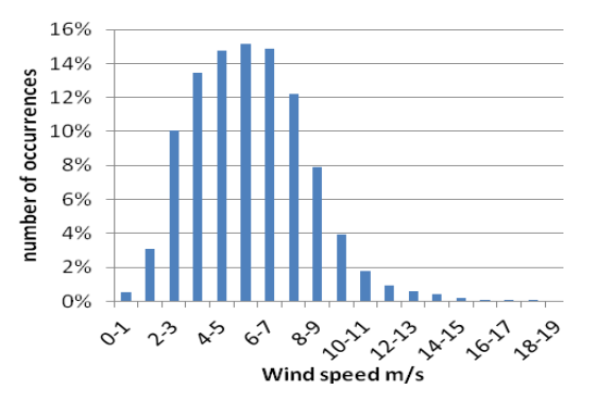
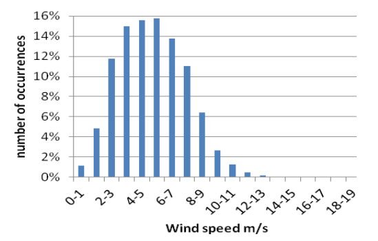
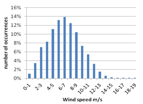
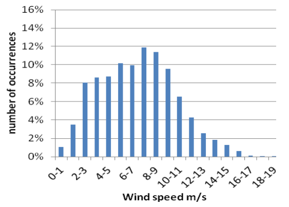
Analyzing the Figures 1-4 differences in wind strength between seasons are noticeable. During the spring and summer wind mostly blows at a speed of 5-6 m/s, during the autumn it increases to 6-7 m/s, while in the winter it reaches even 7-8 m/s. The biggest differences are visible between summer and winter. Although the speed changes to a small extent, it has a significant impact on the quantity of produced energy. Figures 5-6 summarize the frequency and volume of energy depending on the wind direction changing in increments of 15 degrees for two of the most different seasons (summer and winter) when the highest and lowest power outputs are recorded. The distribution of wind directions for both seasons is similar, most of the time the wind blows from the south and south-west.
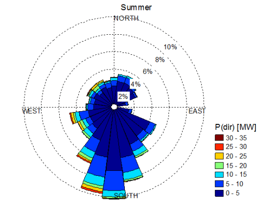
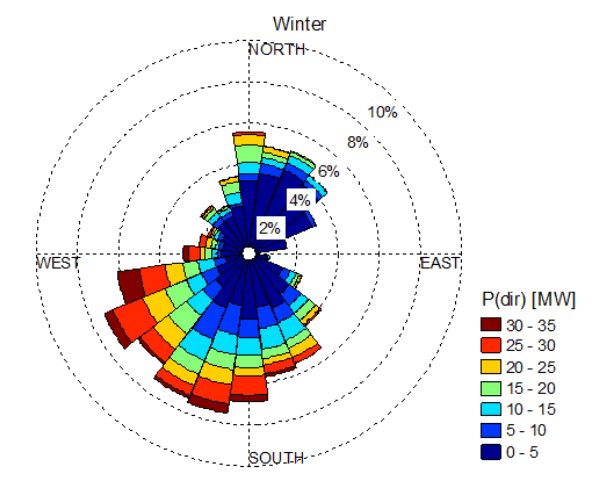
Fig. 5 and Fig. 6 show two of the most different seasons of the year in which the highest and lowest power outputs are recorded. The distribution of wind directions for both seasons is similar, most of the time the wind was blowing from the south and south-west.
The amount of energy production is strongly dependent on the variable wind speed. Figure Fig. 7 and Fig. 8 below are showing the dependence of power on wind speed for summer and winter.
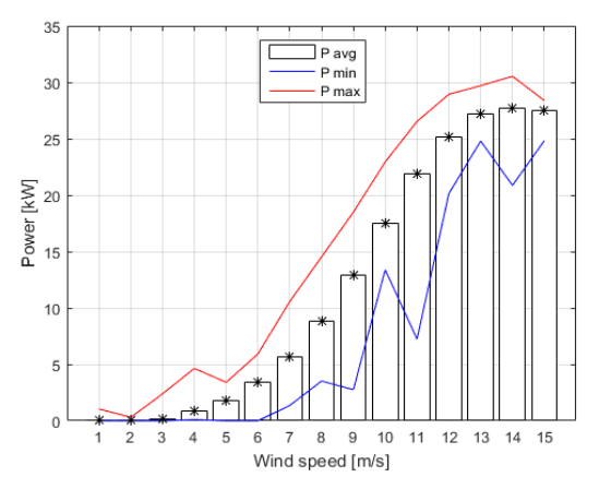
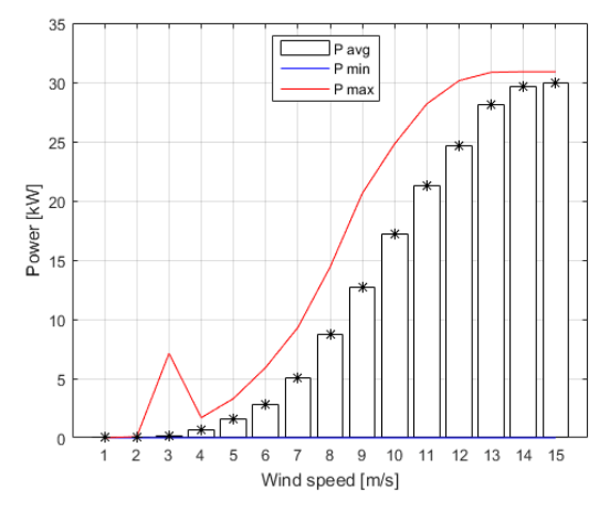
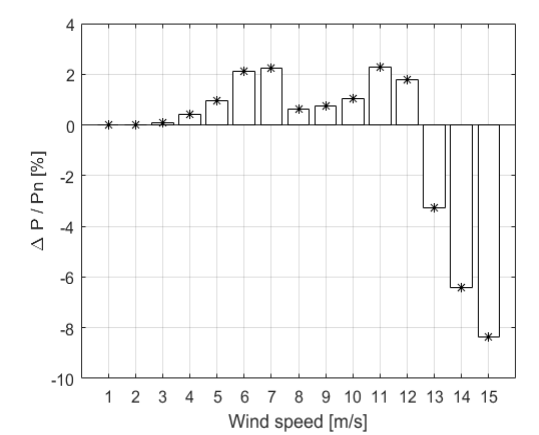
Fig.7 and Fig.8 shows that different average production volumes for the same wind speeds are visible.
As can be seen in Fig. 9 in winter production is on average even higher by 8% for the same wind speed ranges compared to the summer period for wind speeds of 12-15 m/s,. For a smaller wind speed 3-12 m/s the opposite situation is visible.
Wind power can be described by dependence:
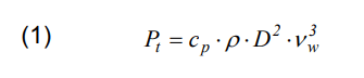
where: Pt – turbine power [W], cp – efficiency, D – diameter of the rotor, ρ – air density.
The wet air density can be expressed by the formula:
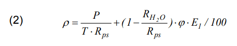
where: ρ – density of air [kg/m3], P – pressure [Pa], T – temperature [K], φ – relative humidity [%], φ=e/E2·100 [%], e – current vapor pressure [Pa], e = E2·φ/100, E1 – maximum vapor pressure [kg/m3], Rps – individual dry gas constant air [J/kg·K], RH2O – individual fixed gas steam [J/kg·K]
As can be seen from the formulas (1) and (2), besides the wind speed there are also other factors that determine the volume of energy production including temperature, humidity or pressure. The table 1 provides additional information about changes to this parameter depending on the season.
Table 1. Summary of characteristic parameters of wind power generation in a seasonal view
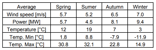
The average wind speed varies slightly depending on the season, the difference is only 1.8 m/s. Bigger differences are observed for parameters like average, minimum and maximum temperature. An undesirable situation is lowering the temperature below 0°C, which may cause icing of windmill blades. This phenomenon changes the aerodynamics of the blades of windmills and it can result in a significant reduction in the generated electric energy, and in extreme cases, it might cause a damage to the fan. Below zero temperatures were registered in autumn and winter. During this period, a strong increase in the average 15-minute power of a wind farm was observed. An increase of 3.6 MW (autumn) and 4.9 MW (winter) compared to the summer, which is over 52% and 70% of the power-to-average power farm for this season.
Unwanted operating states of wind farm
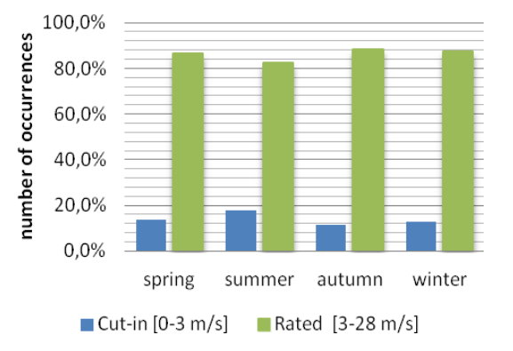
Over the years 2012-2014 the speed of the wind has varied widely. In order to ensure the safety and maximize the efficiency of wind, farm turbines are subject to restrictions due to the speed of the wind. For the considered wind turbines three ranges of wind speed are defined: Cut-in Wind Speed (0-3 m/s), Rated Wind Speed (3-28 m/s) and Cut-out Wind Speed (more than 28 m/s). An analysis of the frequency of farms in these speed ranges for the data from the years 2012-2014 showed no incidents causing an emergency shutdown of the turbine due to too strong wind (Cut-out Wind Speed more than 28 m/s). During vast majority of 15-minute measurements (over 80% of all measurements), wind speed was in the range of normal operation of the wind farm. The differences in the size of the datasets, depending on season, were in the range of ±6,1%.
Because of the climatic conditions in Central Europe, temperatures falling below 0 Celsius degrees, it is necessary to take into account the additional phenomenon of ice on the blades of a windmill. This phenomenon changes the aerodynamics of the blades of windmills and it can result in a significant reduction in the generated electric energy, and in extreme cases, it might cause a damage to the fan.
Building neural models when considering the seasonality
A. Selecting the forecasting models
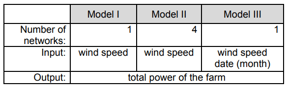
This chapter presents the results of prediction of the power output of an onshore wind farm operating with 15 turbines for three different forecasting models. The learning process of the neural network was performed using back propagation (BP-neural network) and the Levenberg Marquard algorithm. The verification of the models was performed using the real weather data. The training sets were selected in such a way to get two full years, including all four seasons.
The verifying data sets contains measurements from one full year. Various types and structures of artificial neural networks dedicated to the prediction of the energy in wind farms have been proposed in [4]. ANN have an opportunity to expand, because they can work independently or together with another wind power forecasting method. They both are forms of hybrid structures [5]. Model I is a reference point built on the full annual figures. Model II contains four submodels dedicated to each season independently. Model III takes into account seasonal phenomenon in the form of information about the month for which the forecast was made.
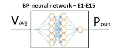
Model I – Pout = f (Vavg)
The first and the simplest model forecasts produced power depending on the average wind speed for the entire wind farm. The operating rules of the neural network Model I are shown in Fig. 11.
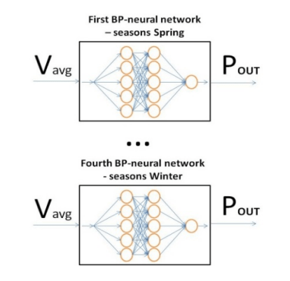
Model II – Pout (seasons) = f (Vavg)
The second model was constructed in a similar way to the first, except that the preparation of four models of learned neural networks using selected data sets for different seasons. As a result, four neural networks for each season separately.
The operating rules of Model 2 are shown in Fig. 12.
Model III – Pout = f (Vavg ,month )
Model III is similar to the model I and, with the difference that the impact of seasonality as an additional input neural network was taken into account as an additional input for neural network. At the input of the neural network the average wind speed for the entire farm and the number of the month for which projections were made introduced.
The operating rules of Model III are presented in Fig. 13.
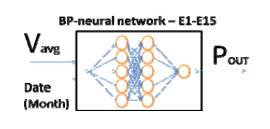
where: Pout – output power of the wind park MW, Date (month) – number of the month for which the forecast was made (ranging from 1-12),
Table 2. Summary of differences between the analyzed models
B. Indicators models
The evaluation of the effectiveness of the models was carried out for a period of one year, by comparing:
• revaluation, underestimation and absolute forecast error
• mean absolute forecast error MAE,
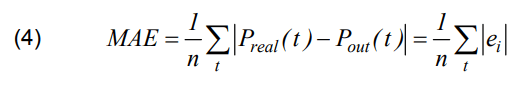
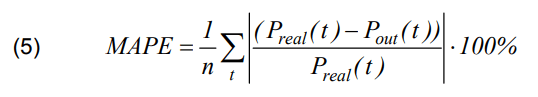
• mean absolute percentage error MAPE
Frequency of obtaining the forecast with the accuracy of 0.75 MW and 1.5 MW, which corresponds to ± 2.5% and ± 5% of the installed capacity of wind
Verification and comparison of models
This chapter presents the results of estimation of electricity production for three proposed models. The prediction was made for an onshore wind farm.
The forecasting method, using artificial neural networks to generate satisfactory results enables the predictions. When considering selection of a variety of structures, a strong dependence of the quality of forecasts on the selected training set was observed. Table II presents the results of forecasting accuracy for each model of forecasting for three models.
Table 3. Summary of results forecasts for the proposed models – the annual results
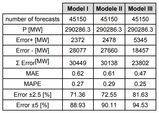
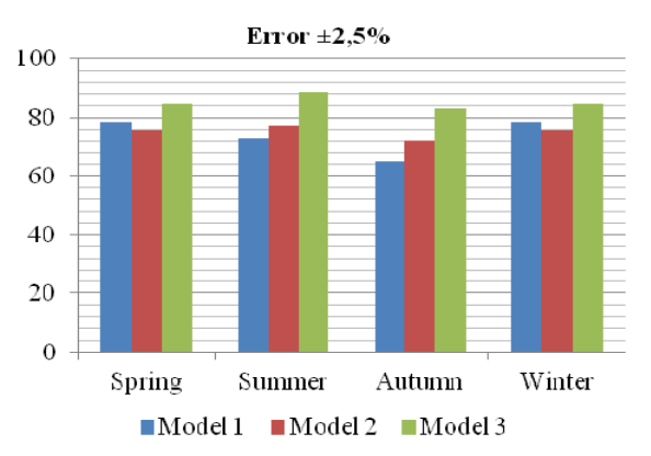
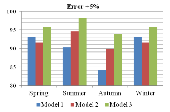
Fig. 14 and Fig. 15 show the results of forecasting accuracy for different seasons:
Conclusion
The long-term electrical and meteorological data from three years of wind farm operation (covering seasonality impact) were used to examine the forecast methods based on three different neural network models.
The analysis of measuring data confirmed the impact of the seasons, and thus the impact of cyclical changes on the energy production volume. The changes of wind speed and temperatures have a significant impact on the operation of the wind farm. The largest volume of energy production was recorded in autumn and winter. The smallest average energy production was registered in summer. Despite an insignificant increase in average wind speed in fall and winter, the average energy production changed noticeably, in the autumn there was an increase of 80%, and in winter, an increase of over 108% compared to summer in which production was the smallest.
Due to the seasonal changes of meteorological phenomena 3 models of neural networks optimized for the impact of seasonality on working wind farm have been proposed and compared. The third model was the best, but it need long-term data. At the of input of the model information about wind speed and the month for which the forecast energy production was carried out, has been given. Such incorporate cyclic phenomena in this case turned out to be most effective. The disadvantage is the need for a large training set to train the neural network. Such a set would allow to prepare a wide range of forecasts of energy from a wind farm. Too little data may result in not full restoration of the power curve of a wind farm. For summer and autumn a bit better was Model II prepared on selected data for individual seasons. For spring and winter the simplest Model I turned out to be slightly better than the Model II.
REFERENCES
[1] Całus D., Oźga K., Popławski T., Michalski A., Szczepański K., Możliwości i horyzonty ekoinnowacyjności – Zielona energia, Wydawnictwo Instytut Naukowo-Wydawniczy “Spatium”, Częstochowa 2018
[2] Popławski, T., Weżgowiec M., Krótkoterminowe prognozy cen na Towarowej Giełdzie Energii z wykorzystaniem modelu trendu pełzającego, Przegląd Elektrotechniczny, 91, (2015), nr 12, 267-270
[3] Ciechulski T., Osowski S., Prognozowanie zapotrzebowania mocy w KSE z horyzontem dobowym przy zastosowaniu zespołu sieci neuronowych, Przegląd Elektrotechniczny, 94, (2018), nr 9, 108-112
[4] Yuan-Kang Wu, Po-En Su, Ting-Yi Wu, Jing-Shan Hong, Yusri M. H., Probabilistic Wind-Power Forecasting Using Weather Ensemble Models, IEEE Transactions on Industry Applications, (2018), 54, 6, 5609-5620
[5] Yang M., Lin Y., Zhu S., Han X., Wang H., Multi-dimensional scenario forecast for generation of multiple wind farms, Journal of Modern Power Systems and Clean Energy, 2015, 3, 3, 361-370
[6] Ciu M., Ke D., Gan D., Sun Y., Statistical scenarios forecasting method for wind power ramp events using modified neural networks, Journal of Modern Power Systems and Clean Energy, 2015, 3, 3, 371-380
[7] Safari N., Chung C. Y., Price G. C. D., Novel Multi-Step ShortTerm Wind Power PredictionFramework Based on Chaotic Time Series Analysisand Singular Spectrum Analysis, IEEE Transactions on Power Systems, (2018), 33, 1, 590-601
[8] M. Qi, G. P. Zhang, Trend Time Series Modeling and Forecasting With Neural Networks”, IEEE Transactions on neural networks, vol. 19, no. 5, May 2008
[9] D. Wu, H. Wang, Application of BP neural network to power predioction of wind power generation unit in microgrid, Engineering Technology and Applications, London 2014.
[10] Z. Liu, W.Gao, Y.-H. Wan, E. Muljadi, “Wind Power Plant Prediction by Using Neural Network”, IEEE Energy Conversion Conference and Exposition, August 2012
[11] Wen-Yeau Chang, “Short-Term Wind Power Forecasting Using the Enhanced Particle Swarm Optimization Based Hybrid Method, Energies, (2013), 6, 4879-4896
Authors: mgr inż. Mateusz Dutka, AGH University of Science and Technology, Department of Power Electronics and Energy Control Systems, 30 Mickiewicza Ave., 30-059 Krakow, POLAND, E-mail: mdutka@agh.edu.pl; dr inż. Bogusław Świątek, AGH University of Science and Technology, Department of Power Electronics and Energy Control Systems, 30 Mickiewicza Ave., 30-059 Krakow, POLAND, E-mail: boswiate@agh.edu.pl.
Source & Publisher Item Identifier: PRZEGLĄD ELEKTROTECHNICZNY, ISSN 0033-2097, R. 95 NR 7/2019. doi:10.15199/48.2019.07.25
