Published by Dušan MEDVEĎ1, Zsolt ČONKA1 Marek PAVLIK1, Ján ZBOJOVSKY1,Michal KOLCUN1,Michal IVANČÁK1, Technical University of Košice, Department of Electric Power Engineering, Mäsiarska 74, 04001 Košice, Slovakia (1)
Abstract. This paper deals with the prediction of electricity generation in particular part of the network (island operation) where were considered various regimes of the wind power plant as a one of the power sources. The simulation network was created in Matlab/SimscapePowerSystem environment that consisted of rotating generators (for regulation of power due to fluctuated wind power generation) and wind power plant of variable energy generation and loads. There were considered the following wind power plant regimes: dynamic wind speed and dynamic load; dynamic wind speed and constant load; constant wind speed and dynamic load. From the all regimes were created prediction diagrams which form the day diagram of load.
Streszczenie. Artykuł dotyczy prognozowania produkcji energii elektrycznej w wydzielonej części sieci pracującej wyspowo, gdzie rozważano różne reżimy eksploatacji elektrowni wiatrowej jako jednego ze źródeł mocy. Sieć symulacyjna, opracowana w środowisku Matlab/ SimscapePowerSystem, składała się z wirujących generatorów (do regulacji mocy z uwagi na fluktuacje generacji wiatrowej) i elektrowni wiatrowej o zmiennej generacji energii i mocy. Rozważano następujące reżimy pracy elektrowni wiatrowej: dynamiczną prędkość wiatru i dynamiczne obciążenie; dynamiczna prędkość wiatru i stałe obciążenie; stała prędkość wiatru i dynamiczne obciążenie. Ze wszystkich reżimów powstały diagramy predykcyjne tworzące dobowy przebieg obciążenia. (Prognozowanie produkcji energii elektrycznej w pracy wyspowej dla różnych trybów generacji wiatrowej).
Keywords: wind power plant, off-grid network, flicker –effect.
Słowa kluczowe: elektrownia wiatrowa, praca wyspowa, efekt migotania.
Introduction
This article presents the particular results of the simulation of the impact of various electricity sources on a small off-grid. Diesel generators and wind turbines have been used as power sources. From the point of view of electricity consumption, the effect of disconnection or connection of a large load on the system and the effect of a dynamically changing load is described. Multiple circuits have been simulated to verify some of the network phenomena. The main monitored variables included network frequency, voltage at the point of consumption, and power produced by sources.
To simulate these phenomena, the Simscape Power Systems, which is an extension of Matab Simulink, was used. Based on the simulation analysis, a simple solution was developed to reduce the impact of transient phenomena. Since simulated transient phenomena of a short nature, i.e. they take a short time, the designed simulations simulate the time interval within 1000 seconds, which is about 17 minutes. A short time interval has also been chosen because the results that are written in matrices have some accuracy and can be processed with current common computing techniques.
Description of the network model of components in the environment of Simscape Power Systems
In the Simscape Power Systems, several electrical machines are implemented. Many of these electrical machines can work in two states – as electricity generators or as motors, that is, as electric consumer appliances [1, 2]. Model of the synchronous machine with expressed poles was used. The synchronous generator is controlled by a hydraulic turbine combined with the PID control system and excited by the AC4A excitation system. The principal scheme of the G1 generator with a control and exciter system and generating output from the generator can be seen in Fig. 1.
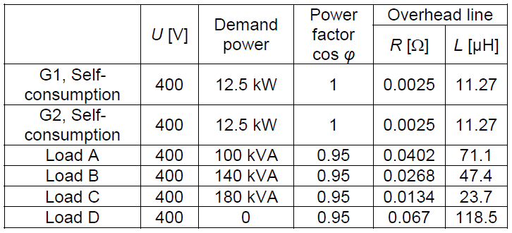
Output of the synchronous generator is a three-phase voltage at the terminals of the machine A, B and C and the measurement output marked with the letter “m”. The measurement output includes a vector with measured signals: stator currents, stator voltages, rotor angle deviation, rotor speed, electromagnetic torque, output active power P, output reactive power Q, and so on. These signals receive feedback from the generator that is input to the exciter winding input and the hydraulic turbine with the control. The label data of the simulated generator are shown in Table 1.

Table 1. Data of the simulated generator.

In Fig. 2 is a model of a hydraulic turbine with PID control. This model has 5 inputs and 2 outputs. Inputs include reference speed, instantaneous mechanical speed, speed deviation, reference power and instantaneous power output. The output is the mechanical power Pm, which is also the input for the synchronous generator. In the mentioned model was set the reference speed ωef = 1 pu, and the inputs of the immediate mechanical velocity ωe and the velocity variation dω were connected. This regulation ensures the regulation of the synchronous generator at the nominal frequency fn = 50 Hz. Inputs of the reference mechanical power Pref and instantaneous power Pe0 are not connected. The circuit is set so that it does not take any feedback (or feedback from the gate output). It has been achieved that the turbine power was controlled only by rotor speed [7].

Wind turbine
The wind turbine block with power-out transmission to the grid is considerably easier than a block of PV field. The wind turbine input is the wind speed reported in m·s–1 and a Trip connector. The wind speed for this model was retrieved from a text file. Trip connector serves to simulate the turbine protection system. Its input may be a logical zero or one. If at input port is logical zero, the wind turbine is in operation and when at input is logical one, the turbine is disconnected. The wind turbine can have several protections. First of all, it is a wind turbine disconnection when there is slow/fast wind, but also overcurrent protection, undervoltage protection, overvoltage protection, or protection, acting in the unbalanced current or voltage.
The wind turbine output is a measuring port that contains the voltage and current at turbine terminals A, B and C, turbine output P and Q, turbine rotor speed, mechanical torque, and so on. The wind turbine used in this article includes, in addition to the turbine, also an asynchronous engine that generates the electrical energy. In Fig 3 is shown the characteristic output of the designed turbine at different wind speeds.

Since during the simulation the disconnection of the wind turbine caused a mathematical error, the block “Check static range” was added to the scheme. This block stops the simulation if a wind speed is read at a speed that is not in the work range, and Matlab shows error message. The wind turbine operating range is in ranges from 4.5 m·s–1 to 12.5 m·s–1. The basic wind speed for the model turbine was set to 9 m·s–1.
Definition of Loads
Simscape Power Systems offers several types of loads. In this article, three-phase serial RLC load and three-phase dynamic load were used. For both loads, the combined nominal voltage and nominal frequency of the network were entered.

For a static three-phase load, PQ power was entered, which may be the same or specific for each load in all three phases. A static three-phase load contains also a voltage and current measurement that is optional [3, 4, 6].
For dynamic three-phase load, the PQ power was entered at the beginning of the simulation. The PQ power of a dynamic load can be controlled by an internal control that controls the amount of dynamic load based on the positive sequence voltage component. If external control of power source is used, performance can be read from a file, and controlled by an external handling. The dynamic load contains also a measuring terminal „m“, the output of which is a vector with a positive-sequence voltage component, an active power P and a reactive power Q [5, 10].

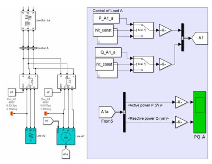
The loads were read using a Matlab script. In Fig 6, a proposed load block for the supply point A is shown. On the left, the load A1 and line A2 are shown, which are connected to the system via a three-phase circuit breaker and a power line simulated by the impedance Ra and La. Line A2 consists of a purely ohmical load, because the dynamic load line A1 cannot be connected in series with the inductive element of the three-phase line, which is the supply point connected to the system. On the right, the reading of block of line load A1 is displayed. If init_const = 1, the load, i.e. line A1 is set according to the vector from a text document. If init_const = 0, the load is set to the constant value, which is set in the text document for time t = 0. Current and voltage measurements were performed on bus-bar A. During the simulations, four consumption points A, B, C and D were considered. Each of these consumption points represents a part of the network. In some simulations, only static three-phase consumption points were used that were disconnected by a three-phase switch.
Measurement in Simscape Power Systems
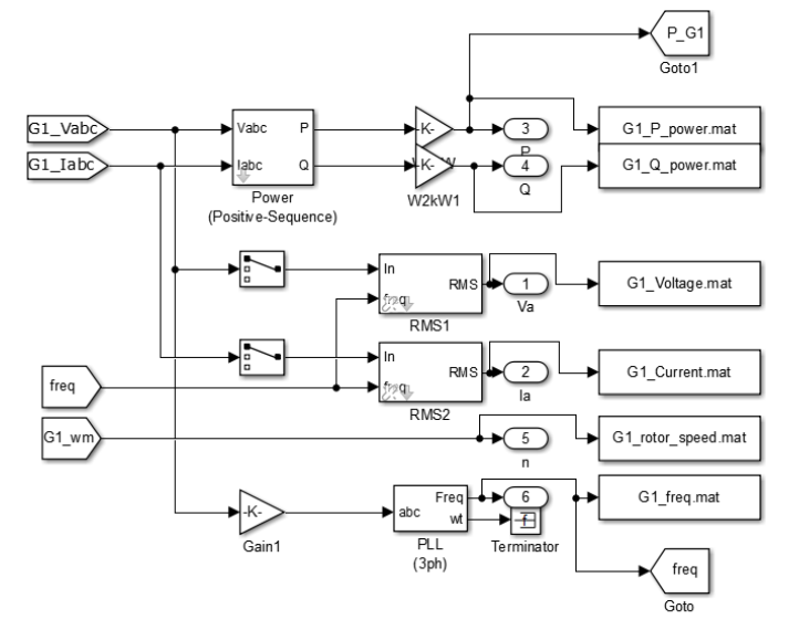
In the simulations, electrical quantities were measured at selected locations in the network. Phase currents and voltages were measured using three-phase V-I measuring blocks, which were placed before loads and before the generators, resp. other sources. The measured output is the sinusoidal voltage/current depending on the time that has to be converted to the effective value (for comparison purposes). The scheme for measuring of the particular variables at the output of the G1 generator is shown in Fig. 7. The RMS current and voltage values for the L1 phase and the active and reactive power in the L1 phase were calculated from the measured currents and voltages.
Model of a steady-state off-grid network

In the off-grid steady-state model, the main aim was to point out that if no changes were made to the scheme and the correct initialization conditions were set, the network’s frequency did not change and was 50 Hz. The phase voltage in phase L1 is equal to the portion of the line-to-line voltage and the square root of 3. If in a system were also considered losses on the line, the resulting voltage values were less than the expected 230 V. In the system were considered large losses on lines, so the phase voltages at the terminals were lower, namely: Ua_A = 220.5 V, Ua_B = 221 V, Ua_C = 223.1 V, and Ua_D = 227 V. The demand current depends on the size of the load being connected at the consumption point (load). The active and reactive PQ load was unchanged in the circuit.
Table 2. Consumptions for simulation of steady-state off-grid network
Model of off-grid network with dynamic load
In this part of the simulation there was modified model of loads. Instead of the loads modeled by the constant value, dynamic loads were used that were controlled by external input. Dynamic load operation is described in the previous chapter definitions of loads During these simulations, two generators with a nominal power of 250 kVA and four loads A, B, C and D were used in which the phase voltage and current in phase L1 and power value in L1 were measured.
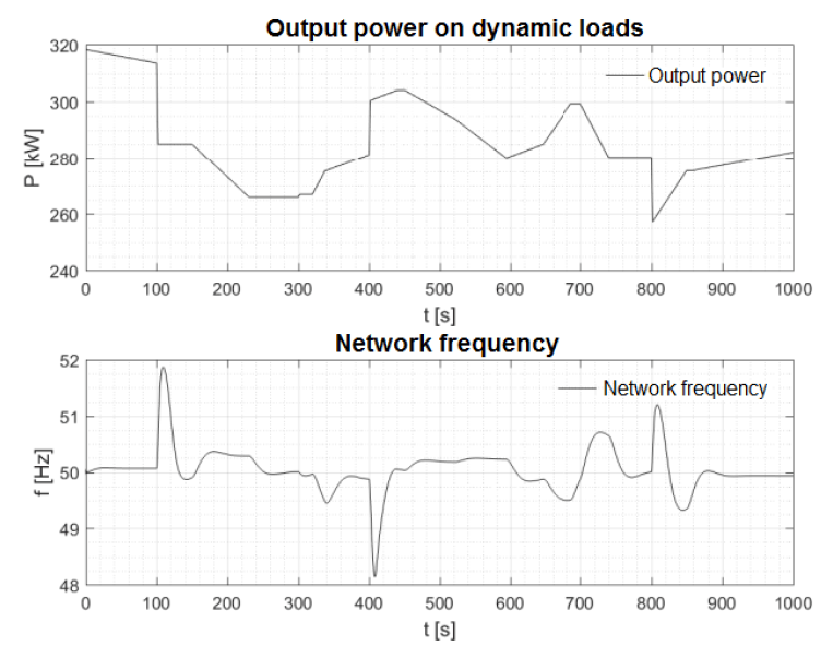
In Fig. 9, the consumed power is indicated by dynamic loads. Self-consumptions (2 x 12.5 kW) and parasitic loads to dynamic loads (3 x 9.5 kW + 4.75 kW), which are purely resistive, have to be added to the total output power. These parasitic loads are in the system because dynamic loads and synchronous generators cannot be in series with an inductive element of three-phase power lines. Those are described by the RL parameters listed in Table 3.
Table 3. Resistance and inductance of power lines in simulations with dynamic load

By a continual decreasing, respectively by increasing of the power consumption there was observed, that the regulators of the synchronous generators respond to these changes, and there is a decrease, respectively increase in output power produced by synchronous generators, but the frequency is not regulated to the nominal value of fn = 50 Hz. Thus, the frequency of the network will be short-lived at a different value near the nominal frequency due to the rate of decrease/increase of the consumed power. This can also be seen in Fig. 9, from 478 seconds to 595 seconds, the network’s frequency was around 50.2 Hz. From 900 s to 1000 s the network frequency was stable at values between 49.93 and 49.95 Hz.
Off-grid model with a wind turbine that operates at a dynamic wind speed
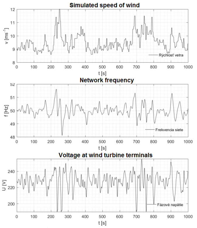
Wind simulation was used to simulate the wind-flow circuit as it is illustrated in Fig. 10. The wind loaded from the text file has a value of 9 m·s–1 at time t = 0, which is the nominal wind for the wind turbine used. Subsequently the wind varies around this value. Wind reaches a maximum value of 12 m·s–1. The wind turbine operates with winds ranging from 4.5 m·s–1 to 12.5 m·s–1.
Since the simulated wind turbine has no stabilizing mechanism, the supplied turbine power also varies around the nominal value. This was reflected negatively on network frequency and voltage. Since the simulated off-grid network is small in size, voltage fluctuations have been registered in all four A, B, C and D loads. Frequency of the grid and voltage at the wind turbine terminals are shown in Fig. 10. Referring to Fig 10 it can be seen that even with small wind changes, the frequency has risen above 51 Hz, or falls below 49 Hz. Voltage at wind turbine terminals is fluctuating. In case of a sudden change of wind, the voltage exceeds 250 V, respectively drops to 190 V. Since the voltage fluctuations are relatively strong, a digital flickermeter has been connected to load points A, B, C and D and to the wind turbine connection point.
Flicker-effect measurement in network with a wind turbine
In the previous section there was a description of offgrid operation with a wind turbine with dynamic wind. In order to determine the flicker effect in the aforementioned network, a digital flickermeter was added at points A, B, C and D to find a short-term flicker rate that is calculated at simulation time of 5 to 605 s, representing a ten-minute time period. In Table 4 is the measured short-term rate of flicker and averaged percentiles. The smallest rate of flicker shortterm perceptive was simulated with a constant wind velocity of 9 m·s–1 and a dynamic load. On the other side, the highest short-term flicker rate was simulated with dynamic wind speed and dynamic load. The short-term flicker rate was in accordance with standard STN EN 50160.
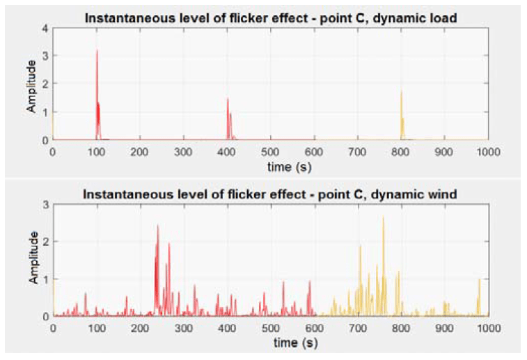
The Fig 11 shows the measured instantaneous level of the flicker effect at the load point C for dynamic load simulation (Fig. 9) and the dynamic wind simulation (Fig. 10). From Fig. 11, it is apparent that the blink effect was occurred in the case of dynamic load simulation at a time when the load was connected or disconnected in the network. It was observed for example, at time t1 = 100 s when a load of 30 kVA was disconnected at the load point B or at time t2 = 400 s when a load of 20 kVA was connected at the load point C or at time t3 = 800 s when the load of 20 kVA was disconnected from load point C. In the case when the dynamic wind acts on the wind turbine (see Fig. 10), the measured instantaneous level of flicker effect will appear as a stochastic noise.
The Table 4 shows the short-term flicker rate response for the load points A, B, C and D and for the point on the wind turbine terminals. The particularity of these results is that in each simulated scheme, at the load point A, the highest degree of short-term flicker is measured. This is due to the fact that the point A is powered by a line whose resistance and reactance is much larger than the lines connecting the other points (see Table 3). The voltage at point A in these simulations was stabilized at U = 189.6 V (in real conditions, such a low voltage would be a problem for the operation of many devices).
Table 4. Flicker effect in the simulated network

In order to reduce the influence of power line on the measured flicker effect, the simulations were repeated except that the line joining the load point A was simulated by resistance Rc = 0.0134 Ω and inductance Lc = 23.7 µH connecting the load point C. The results are given in Fig. 12.
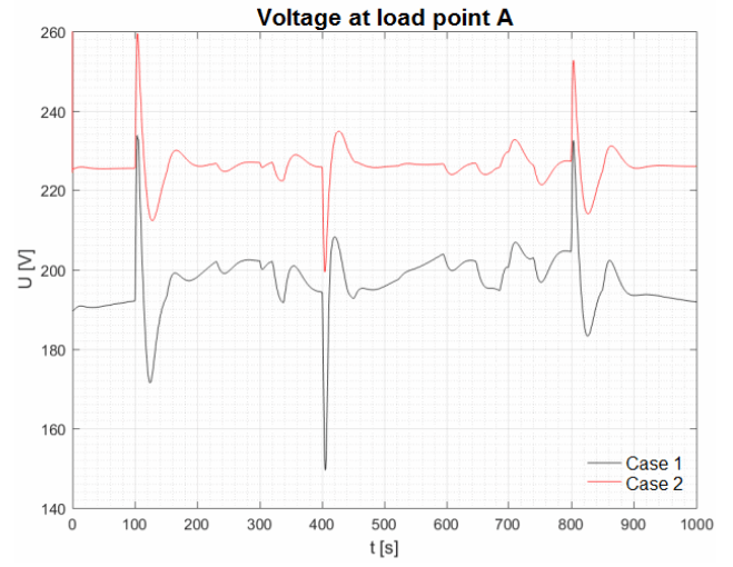
In Fig. 12 is the voltage characteristics at the load point A in the case where was considered constant wind of 9 m·s– 1 during the whole simulation and the dynamic load as described in section B. For the case 1 there was considered the original power line whose resistance was Ra = 0.2010 Ω and inductance La = 355.5 µH. In case 2, a point A was connected by a line with parameters Ra = 0.0134 Ω and La = 23.7 μH. From Fig. 12, it is clear that in case 1 there is a greater voltage fluctuation at the terminals at the load point A as in case 2. For example, during the disconnection of the 20 kVA load from the load point C, there was observed (in case 1) at the load point A the short-term voltage drop from Uf = 194.3 V to Uf = 149.5 V, which is a drop of ΔU = 44.8 V. In case 2, there was drop from Uf = 225.7 V to Uf = 199.4 V, which is drop of ΔU = 26.3 V. As there is less voltage fluctuation in transient phenomena, the resulting flicker effect will be less. In test example 2, the value of the Short Term Perceptibility (Pst) of flicker effect in point A was Pst = 0.335491 (the original value, in case A was Pst = 0.523317).
Conclusion
This article presented the particular results of off-grid network simulations with consideration of renewable resources (wind turbine) and without considering renewable energy sources. The simulated off-grid network consisted of two diesel generators with a nominal output of 250 kW and with loads A, B, C and D, representing 4 load points representing 4 off-grid sites. In the case of a load disconnection or connection, the generators are able to regulate the system so that the power output is equal to the power delivered. The regulation of diesel generators has ensured the control of the hydraulic turbine.
The problem of off-grid systems with a wind turbine (WT) is that the power output from the WT cannot be regulated. The WT produces electricity according to current climatic conditions. Therefore, in the case of rapid climate change, there is a rapid change in the output of the WT. For example, with decreased wind speed, a sudden drop in the electricity produced from the WT may occur. By adding a wind turbine into an off-grid, an increased flicker effect was observed. In addition to voltage fluctuations in the network, the network frequency also varies. Large frequency fluctuations can have a negative impact on diesel generators. Flicker effect occurs when disconnecting or connecting loads, resources, and off-grid networks. In both cases, it is necessary to consider how to remove the unfavorable phenomenon of blinking. For this reason, it is necessary to have good data for prediction of electricity production in island operation under the different wind generation modes.
Acknowledgement This work was supported by the Ministry of Education, Science, Research and Sport of the Slovak Republic and the Slovak Academy of Sciences under the contract No. VEGA 1/0372/18.
REFERENCES
[1] M. Špes, Ľ. Beňa, M. Kosterec, M. Márton, Determining the current capacity of transmission lines based on ambient conditions, In: Journal of Energy Technology. Vol. 10, no. 2 (2017), p. 61-69. ISSN 1855-5748
[2] R. Cimbala, L. Kruželák, S. Bucko, J. Kurimský, M. Kosterec, Influence of Electromagnetic Interference on Time-Domain Spectroscopy of Magnetic Nanofluids, In: EPE 2016. Danvers: IEEE, (2016), p. 279 – 282. ISBN 978-1-5090-0907-7
[3] D. Medveď, O. Hirka, Investigation of Electromagnetic Fields in Residential Areas. In: Acta Electrotechnica et Informatica. Vol.17, No. 3 (2017), p. 48-52. ISSN 1335-8243
[4] T. Košický, Ľ. Beňa, Optimizing deployment of battery storage systems, In: Current Problems of Maintenance of Electrical Equipment and Management. Košice: TU, 2014 p. 131-141. ISBN 978-80-553-1818-9
[5] V. Volokhin, I. Diahovchenko, V. Kurochkina, M. Kanálik, The influence of nonsinusoidal supply voltage on the amount of power consumption and electricity meter readings, In: Energetika. Vol. 63, no. 1 (2017), p. 1-7. ISSN 0235-7208
[6] Z. Čonka, M. Kolcun: Impact of TCSC on the Transient Stability In: Acta Electrotechnica et Informatica. Vol. 13, no. 2 (2013), p.50-54. – ISSN 1335-8243
[7] MathWorks, Model hydraulic turbine and proportional-integralderivative, https://www.mathworks.com/help/physmod/sps/powersys/ref/hydraulicturbineandgovernor.html
[8] MathWorks, Three-Level Bridge, https://www.mathworks.com/help/physmod/sps/powersys/ref/threelevel bridge.html
[9] MathWorks, Av. Model of a 100-kW Grid-Connected PV Array, https://www.mathworks.com/help/physmod/sps/examples/average-model-of-a-100-kw-grid-connected-pv-array.html
[10] MathWorks, Implement three-phase dynamic load with active power and reactive power as function of voltage or controlled from external input, https://www.mathworks.com/help/physmod/sps/powersys/ ref/threephasedynamicload.html
[11] Ž. Eleschová, A. Beláň, B. Cintula, B. Bendík, Smart grids analysis – View of the transmission systems voltage stability, In EPE 2018. Brno: University of Technology, 2018, p. 37-42. ISBN 978-1-5386-4612-0
[12] D. Kaprál, P. Braciník, M. Roch, M. Höger, Optimization of distribution network operation based on data from smart metering systems, Electrical Engineering, Vol. 99, Issue 4, Springer, New York, USA, 2017, December, pp: 1417-1428, ISSN 0948-7921
Authors: Ing. Dušan Medveď, PhD. Technical University of Košice, Department of Electric Power Engineering, Mäsiarska 74, 04001 Košice, Slovakia E-mail: dusan.medved@tuke.sk; Ing. Zsolt Čonka, PhD. Technical University of Košice, Department of Electric Power Engineering, Mäsiarska 74, 04001 Košice, Slovakia E-mail: zsolt.conka@tuke.sk; Ing. Marek Pavlík, PhD. Technical University of Košice, Department of Electric Power Engineering, Mäsiarska 74, 04001 Košice, Slovakia E-mail: marek.pavlik@tuke.sk; Ing. Ján Zbojovský, PhD. Technical University of Košice, Department of Electric Power Engineering, Mäsiarska 74, 04001 Košice, Slovakia E-mail: jan.zbojovsky@tuke.sk; Dr.h.c. prof. Ing. Michal Kolcun, PhD. Technical University of Košice, Department of Electric Power Engineering, Mäsiarska 74, 04001 Košice, Slovakia E-mail: michal.kolcun@tuke.sk; Ing. Michal Ivančák, Technical University of Košice, Department of Electric Power Engineering, Mäsiarska 74, 04001 Košice, Slovakia E-mail: michal.ivancak@tuke.sk
Source & Publisher Item Identifier: PRZEGLĄD ELEKTROTECHNICZNY, ISSN 0033-2097, R. 95 NR 7/2019. doi:10.15199/48.2019.07.31
