Published by Abdelkader BOUDERBALLA1, Boubakeur ZEGNINI2, Tahar SEGHIER2,
Abderrahmane TALEB Higher Normal School (ENS) of Laghouat (1), Amar TELIDJI University of Laghouat (2)
Abstract. The protection of the equipment, the safety of persons and the continuity of the electrical supply are the main objectives of the grounding system. For its precise design, the possible potential distribution on the ground and the equivalent resistance of the system must be determined. Grounding systems are considered to be rod electrodes and flat electrodes buried vertically in the ground. A simulation grounding model was established through FEM method on relevant constraints, such as soil resistivity, number, position and length of electrodes. Through this study, the grounding resistance values obtained with COMSOL Multiphysics are compared with the proven analytical formulas. The results indicate that this simulation can be used as fast solution for industrial applications and has acceptable results for calculating the resistance of a vertical grounding.
Streszczenie. Ochrona urządzeń, bezpieczeństwo osób i ciągłość zasilania elektrycznego są głównymi celami systemu uziemienia. W celu dokładnego zaprojektowania systemu należy określić ewentualny rozkład potencjału w ziemi i równoważną rezystancję systemu. Za systemy uziemienia uważa się elektrody prętowe i płaskie zakopane pionowo w ziemi. Symulacyjny model uziemienia został ustalony metodą FEM na podstawie odpowiednich ograniczeń, takich jak rezystywność gruntu, liczba, pozycja i długość elektrod. Dzięki temu badaniu, wartości rezystancji uziemienia uzyskane za pomocą COMSOL Multiphysics są porównywane ze sprawdzonym wzorami analitycznymi. Wyniki wskazują, że symulacja ta może być wykorzystana jako szybkie rozwiązanie do zastosowań przemysłowych i daje akceptowalne wyniki do obliczania oporności uziemienia pionowego. (Określanie rezystancji uziemienia z zastosowaniem metody FEM)
Keywords: grounding resistance, finite element method, soil resistivity.
Słowa kluczowe: rezystancja uziemienia, metoda elementów skończonych, rezystywność gruntu gruntu.
Introduction
For several decades, research has been intensifying in the field of the ground of electrical installations. The vast majority of this research was aimed at behaviors of these groundings at industrial frequency and under steady state conditions. In addition, the resistivity of the soil considered was generally close to 100 Ω.m (value often in temperate regions), which is not the case in the tropics in certain types of soil. Soil resistivity can reach several thousands of ohms meters. The study of the behaviour of the earth network requires a previous analysis of the distribution of the electric potential in the surrounding soil. This distribution is a function of the electrical characteristics of the ground, i.e. its resistivity (to a lesser extent its permittivity too), the geometrical characteristics of the ground network and the source. The design of an earth network must therefore be preceded by an investigation.
The safety, reliability and correct operation of the power system depend on the design and construction quality of your grounding system [1]. The construction project aims to protect the equipment and personnel of the electrical system from the danger of electric shock. The grounding system can include only one grounding electrode or the entire electrode group. In many of the applications, low grounding resistance is essential to meet electrical safety standards [2].
The grounding resistance is often called the earth resistance. Grounding resistance is defined as the relationship between the voltage on the grounding device and the current flowing to the earth through the grounding device. The value of the earthing resistance is an important technical parameter related to the safety of personnel and equipment. If the earth resistance is high and earth current occurs, it can result in death or personal injury and equipment damage. The value of the earthing resistance at a certain value of the grid current determines the value of the dangerous voltage inside or around the substation.
The main purpose of designing the grounding system of a substation or power plant is to provide safety to personnel in the event of a ground fault. The primary purpose of the electrical system substation is to maintain reliable operation and provide protection to personnel and equipment in the event of failure. The basic configuration of the grounding grid is composed of round steel that forms a two-dimensional grid (usually square or rectangular) and is buried close to the earth surface. The ground rods are only effective if a significant portion of their length is in contact with a low resistivity soil. From the point of view of the safety of people and equipment, there is no doubt that the ground door is the most important part of the electrical system. The reliability and availability of the electrical system depends on the quality of the design and construction of the grounding grids.
The main objectives of the grounding system are:
• Protect personnel from electrical hazards by limiting overvoltage that can be found in the event of a failure in the electrical system.
• The safety and continuity of electrical equipment by limiting the overvoltage that can occur in extreme conditions or accidents.
• The correct operation of the equipment and electrical protection equipment allows detecting faults and selecting all the measures destined to disconnect areas of equipment due to ground fault current.
The calculation method used to simulate the grounding grid considers the following simplified assumptions:
• The soil is an infinite, flat, isotropic and multilayer environment.
• The electromagnetic method is suitable for calculating the grounding resistance and the lattice potential.
• The ground network conductors are considered linear, connected to each other and buried near the surface of the earth.
• The behavior of the earthing grid at the estimated operating frequency can be determined by electromagnetic field analysis techniques for fixed fields (the propagation time can be ignored).
The different methods of calculating the grounding resistance are based on determining the potential or capacitance of the grounding electrode. The method of calculating the grounding grid uses different mathematical techniques to determine the grounding resistance and the step voltage and contact voltage, applying the hypotheses that allow us to model the real system in other theoretical of comparable results. These studies are generally performed on the ground mesh with symmetry and uniformity [2] or two or more layers [3] – [7]. The initial method was based on calculating the earth fault current (amps) from the random grid potential and obtaining the earth resistance value as the ratio between voltage and current. After calculating the earth resistance, the actual grid potential (calculated as the product of the actual fault current and the calculated earth resistance value) is again used to analyze the finite element model to obtain the potential distribution in the model and the touch voltage and the step voltage order.
Recent studies based on the finite element method (FEM) have been used to calculate the ground resistance of earth systems [8],[9] FEM allows to obtain the grounding resistance as a function of the resistivity of soil . Therefore it is possible to justify the use of FEM in the dimensioning of the grounding systems. The FEM method is used to evaluate the solution of the partial differential equation that governs the behavior of the system. The grounding system is considered to be a rod electrode buried vertically in the ground. Earth resistance is also determined using FEM and with calculating the dissipated power or from the stored energy. Then, by integrating the potential distribution on ground surface, current density distribution inside soil, we finally calculate the amplitude of the current passing through the earth rod or region, the ground resistance is determined as the ratio between the voltage and the calculated current. In this paper , we will propose a simple model of calculation by FEM to evaluate the impulse characteristics of the soils, coming as close as possible physical realities. This method will allow us to study the effect of certain parameters (soil resistivity, geometric positions of the electrodes) on performance of grounding systems in order to propose concrete solutions for the best realization of earthing systems, respecting the standards for the safety of equipment and people.
Material and Method
The latest research on fundamental analysis is based on the finite element method. The design of the earthing system using the FEM method aims to determine the earth resistance. Compared to the traditional soil method, the finite element method provides more accurate results [8]. The oldest FEM method consists of current analysis using the electrode potential. Once the current is calculated, the ground resistance can be found by dividing the voltage by the current. In this method, the main disadvantage is that the size of the model is chosen as a considerable ground distance from the ground electrode. Because the earth electrode of the grounding point considers the analysis of each potential in the grounding of the selected point.
Where: From tests of various designs, d1 can be determined by:
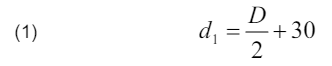
where: D is the diagonal distance of grounding electrode, d1 is the distance from electrode to the points where semispherical model of equipotent surface distribution.
Resistance of grounding electrode can be derived from Fig.(1):

where R1 is the resistance inside the semispherical surface, R2 is the resistance outside the semi-spherical surface.
Resistance R2, ground resistance between d1 and infinite, which is small compared to, can be calculated by applying expression (3) to calculate the resistance of a semi-spherical resistor of internal radius and infinite external radius see Fig( 1). R2 is computed from the following equation

where: ρs the soil resistivity

The R1 ground resistance of a semi-sphere with radius d1 (see Fig. (1)).Being d1 the earth distance for which the distribution of potentials can be supposed spherical.
This is where finite element analysis exactly takes its place. In general, R1 can be calculated from dissipated power given in the following equation:

R1 can be detailed by replacing the terms as in Equation (4)

where: VG is the potential in the grounding electrode; VB is the potential in the boundary d1; E is the electric field; dV is the volume element; σ is the electrical conductivity.
At the same time, dissipated power is determined by :
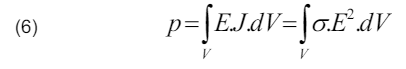
Dissipated power (6) is calculated by applying current flow analysis to the finite-element model. The finite-element model is comprises d1 of a semi-spherical volume of radius Fig. (1) and is defined according to the geometry of the grounding grid and the soil structure.

where: V is the electrical potential; σ is the electric conductivity, je is the external current density and Qj is the current source density.
In the proposed method, the ground around the rod is divided into three cylindrical shaped parts as shown in Fig. (2). It is believed that the first cylinder, referred to as the grounding system, has a radius of 2.5 times the length of the rod to maintain a sufficient volume of the beam to guarantee efficient current discharge.
The second cylinder, called the effective soil, is usually considered to have a radius and a height of 10 m. The next layer or the third cylinder with a height and a radius of more than 10 meters, which does not have a significant effect on the soil resistivity, is considered to be infinite.
The cylindrical electrode, although it is not really used, has great importance in the study of grounding systems since equipotential surfaces of any grounding rods become hemispheric at a sufficiently long distance form the rods themselves. Therefore, it is possible to approximate any shaped rod with a cylindrical electrode having an equivalent radius.

FEM is known with its unique triangles. Initializing the mesh allows the designer to see the triangles made by the COMSOL multiphysics solver, which is shown in Fig. (3).
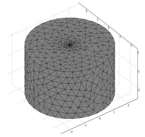
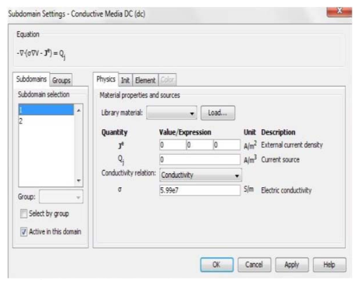
Table 1.Subdomain for the rod electrode and Soil

The boundary conditions define the interface between the geometry of the model and its environment. You can also set the interface conditions on the internal limits of the model geometry. Different boundary conditions can be defined for each boundary is shown in Fig. (5).
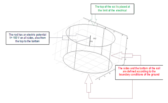
You can also define different boundary conditions for each limit. For the bar, the potential limit is defined as V0 = 100 V. It should be noted that the surrounding soil actually has infinite dimensions. Therefore, it is possible to model with a domain whose size is much larger than the size of an earthing system with boundary conditions set to zero potential.
For the soil, the boundaries are selected as follows:
• From conditions shown in Fig. (2), the four sides, and the bottom of the soil cylinder were set to ground boundary condition.
• The top of the soil cylinder was set to electrical insulation boundary. This model is the model governed by Laplace equations, which is the governing equation for the earthing system under design. Dependent variable is by default set to 100 V, which is the behavior parameter to be studied and analyzed. At industrial frequencies, the ground connection is modeled by resistance.
To obtain the Laplace equation final solution, simply clicking the Solve button on the Main toolbar yields the solved model.

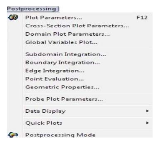


To calculate the power loss, the following steps from Fig (6) to Fig (9) have been performed:
1-Select Finishing in the menu bar;
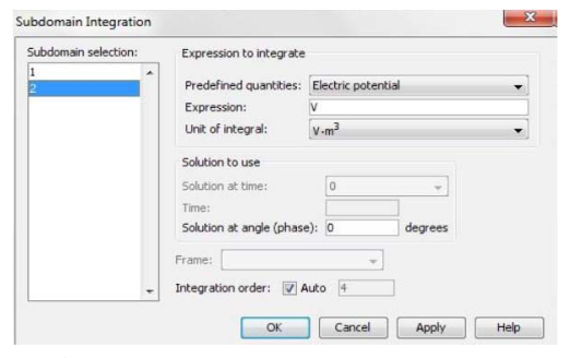
2-From selection after processing to subdomain integration, the Subdomain Integration dialog box opens;
3-Selection of resistive heating from the predefined quantities with remaining values Select subdomain 1 in the subdomain integration dialog
4-By pressing OK, the resistive heating in the bottom medium is calculated, which represents the power loss between the pole edge and the bottom limit;
5-Review the results while viewing the message log to see the results in the drawing area at the bottom of the message log.
The dissipated power is calculated using this software by integrating the appropriate domain for the predefined quantity of resistive heating. The domain of the soil has been chosen to calculate the dissipated power between the rod edge and the outer boundary of the soil. Resistive loss is chosen by clicking the volume integration button in the software window, and the value of the resistive loss is found. To obtain the ground resistance of the earthing system from COMSOL Multiphysics we use the resistive heating integration in the Subdomain of soil, to get the dissipated power from the rod in the soil around it, and the resistance R1 is equal to the square of the voltage of rod over this power, a detailed calculation can be found in the reference [12].
Simulation Results and Discussion
The results obtained by the COMSOL program package based on FEM are given. COMSOL is software for various physics and engineering applications (especially related phenomena or multiphysics). For comparative analysis, the AC / DC module is used in conjunction with the “current” interface. The geometry of the ground system is modelled based on the actual geometry of the grounding system.
The rod, is designed as a cylindrical shaped element with radius r, and length l, and made of copper with conductivity of copper that is σ = 5.99 107 (Ω. m)−1 or resistivity of copper which is ρ = 1.66 10-8 (Ω .m). The rod is driven vertically into the soil.
For the evaluation, we will start with a simple hemispherical electrode. The soil is represented by a hemisphere with a large radius (towards infinity). First, to simplify the calculation, let’s consider homogeneous soil. The calculation will be done in asymmetric situations and in 3D.
Next, we will consider several layers of soil with different resistivity’s. The model used is identical to the one that the soil has a single layer; the analytical relations depend on the length of the electrode in relation to the depth of the layer Fig (11).
A two-layer soil model is generally used for nonhomogeneous soil characterizations. The first layer thickness is h = 5.5 m with a specific resistivity of 1000 Ω. m, where the second layer with resistivity is 100 Ω. m, the calculations were carries out in 3D and axi-symmetric.

In all simulations, a 10 A current has been injected into the ground rod in order to evaluate the potential on the earth surface from the rod itself to a sufficient long distance characterized by a null the ground potential.
The computations are conducted in axi-symmetric Fig. (12) shows the possible potential distribution of a 10 A current flowing through a 4 m long electrode.

For a cylindrical copper electrode of radius 0.0125 m, in a homogeneous soil of resistivity 100 Ω.m, the grounding resistance is given by the Fig (13), as a function of the length of the electrode, in axi-symmetric and 3D. Also represented on this graph are the resistances calculated with the analytical relationships of Rudenberg, DwightSunde and Liew-Darveniza (see Table 2).
Table 2. Analytic equation of the grounding resistance

With ρs the resistivity of the soil, l the length of the electrode and d the diameter of the electrode, r the radius of the electrode.

The relative errors considering that the analytical relation Dwight–Sunde is exact are indicated below on the Fig. (13), these curves show us that the modeling which we have chosen is adapted to a cylindrical electrode. The errors are less than 10% compared to the analytical calculations Fig. (14).

We also note that analytical relationships of DwightSunde and Liew-Darveniza give more accurate results, close to those obtained by finite elements, the axisymmetric calculation being more precise than the 3D.
As for the cylindrical electrode, the 3D calculation is very expensive in term of computing time and resources. For copper electrodes of radius r = 0.0125 m, the distance between electrodes being equal to twice their length, and for a resistivity of 100 Ω.m, the resistance of the set of two stakes in line and the relative error by considering analytical equation of Dwight-Sunde gives results closer to those calculated by finite elements, with relative errors of less than 5%.
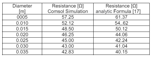
According to the standard, improving the grounding system means that the resistance of the grounding system is reduced. For this reason, an effective way to reduce resistance must be found. We will list these different resources and assess the impact of improving their authorized grounding. In this evaluation, we will always calculate the ground potential after current injection, then we can deduce the resistance value from it and compare it with the literature [13],[14].
Table 3. Resistance as a function of the diameter of the vertical cylindrical electrode
To achieve low resistance, a single vertical electrode is usually not sufficient. It is important to use several electrodes in parallel. Fig. (15) and Fig. (16) show the ground potential and the earth resistance depending on the number and distance between vertical cylindrical electrodes 2 m length, and r = 0.0125 m with a current of 10 A with soil resistivity of 100 Ω.m. Tables 3 and 4 show the effect of increasing the number and distance of electrodes on the grounding resistance.
Table 4. Resistance as a function of the distance between the 4 cylindrical electrodes


For example, when changing from one electrode to 4 electrodes, the resistance is divided almost by four. We realize that when changing from one electrode to two electrodes, the resistance can be minimized, which means that it is efficient, but takes up space, and increase installation costs.
According to the results in Table 4, we noticed that the grounding resistance decreases as the distance between the four earth stakes increases. For example, if the distance goes from 2 m to 4 m, the ground resistance decreases by 12. 36%, while that from 2 m to 10 m, the decrease is only 20%. This shows once again that for cost and space considerations there is a limit to the distance between the electrodes. The literature reports that the 6 m distance between the electrodes is economically a limit to the cost of grounding [13].The impact of resistivity on the grounding resistance for an electrode of l = 2m, r = 0.0125m through which a current of 10A flows in a soil of different resistivity (10 Ω.m, 100 Ω.m, 1300 Ω.m) are represented by Fig. (17). Differences in results of calculations and simulations were caused by simplifications adopted in calculations.

In high resistivity soils, the conductivity of the earth conductor is less than that of low resistivity soil, making it difficult for the earthing system to dissipate the current injected into soil. Resistivity can be reduced by treating the soil with charcoal and other products such as wood bentonite and salt [5].The IEC 62305-3 standard deals with the protection, inside a structure, against physical damage and against injury to living beings due to touch and step voltages. The essential and most reliable protective measure for the protection of structures against physical damage is considered to be the lightning protection system 18]. Main protection measures against injury to living beings due to touch and step voltages are intended to: reduce the dangerous current flowing through bodies by insulating exposed conductive parts, and/or by increasing the surface soil resistivity. Using durable materials to ensure long, continuous operation. In dry soil, but in corrosive acid, salty, or humid environments require regular maintenance. Soil resistivity depends on the content of electrolytes in the soil, geological and chemical considerations and seasonal variations in a site. In different seasons, the resistivity of the surface soil layer will change, which will affect the safety of grounding system, and the grounding resistance, step and touch voltage will move to the safe side or to the hazard side. In this evaluation we will always calculate the potential in the earth after the injection of the current, then we can deduce the value of the resistance and we compare it with the analytic expressions.
Conclusion
The purpose of this work was to define an alternative method for assessing earth resistance with FEM methods. This method makes it possible to take into account more specific cases than what the standards formulas (calculations according to fundamental formulas) for calculating the earth resistance of different ground electrodes. The model was validated by comparing the well-known equation of ground resistance for a vertical cylindrical electrode with one simulated by FEM analysis.
In this study, in order to evaluate the grounding resistances (also the electric field and potential distribution and current density) in industrial frequency, the finite element calculation models were presented in 2D axisymmetric and 3D, for some electrode configurations. These calculation models, which have the advantage of being closer to the actual physical situation, and which apply to more complex configurations have been validated against analytical calculations, with differences in relative error low and often in the order of 10%. These results showed that axi-symmetric calculations are much cheaper in terms of calculation time and resources because they allow much finer meshing. The ground resistance should be as low as possible to ensure the safety of personnel and equipment. The presented FEM method is very useful for calculating grounding resistance as a function of the resistivity of soil. Then, it will be possible to justify the use of this method in dimensioning of the grounding systems.
A future development of this work may be the study of the frequency variation, especially the behavior of the earth for high-frequency components that characterize power electronic devices or telecommunication systems.
Acknowledgments: This work was financially supported by Directorate General for Scientific Research and Technological Development (DGRST) Ministry of Higher Education and Scientific Research Algeria, under the Scientific Program/ PRFU. Contract/, No A01L07UN030120180002.
REFERENCES
[1] Hyung-Soo L., Jung-Hoon K., Dawalibi F. P., and Jinxi,,M. “Efficient ground grids designs in layered solids,” IEEE Trans. Power Del., vol. 13, no. 3, pp. 745–751, Jul. 1998.
[2] Thapar B., Gerez V., Balakrishnan A. and Blank D. A. “Evaluation of a grounding grid of anyshape”, IEEE Trans. on Power Delivery, Vol. 6,No. 2, pp. 640-645, April 1991.
[3] Dawalibi F. P. and Mukhedkar D., “Optimum design of substation grounding in two-layer earth structure”, IEEE Trans. Power Apparatus and Systems, Vol. PAS-94, No, 2, pp. 252-272, April 1975.
[4] Seedher,H.R. Arora J.K. and Thapar B., “Finite expressions for computation of potential in two layer solid”, IEEE Trans. on Power Delivery, pp.1098-1102, 1987.
[5] Lee H.S., . Kim J.H, Dawalibi F.P. and Ma J., “Efficient ground grid designs in layered soils”, IEEE Trans. On Power Delivery, Vol. 13, No. 3, pp.745-751, July 1998.
[6] Thapar B.. and Goyal.S.L., “Scale model studies of grounding grids in Non-uniform soils”. IEEE Trans. on Power Delivery, Vol. 2, pp. 1060-1066, October 1987.
[7] Takahashi T. and Kawase T., “Calculation of earth resistance for a deep-driven rod in a multi-layer earth structure”, IEEE Trans. On Power Delivery, Vol. 6, No. 2, pp. 608-614, April 1991.
[8] Nenad N. Cvetković, Dejan B. Jovanović, Aleksa T. Ristić, Miodrag S. Stojanović, Dejan D. Krstić, Comparison of different models for determining the grounding rod resistance, ELECTROTECHNICA & ELECTRONICA, (E+E), Volume 50, Issue 9-10, 2015, p p.35-39. 2015.
[9] Sajad Samadinasab, Farhad Namdari,Mohammad Bakhshipour, A Novel Approach for Earthing System Design Using FiniteElement Method, Journal of Intelligent Procedures in Electrical Technology, Vol. 8 – No.29 – pp54-63 Spring 2017.
[10] AbuBakar,A. Dow R.S., “Simulation of ship grounding damage using the finite element method”, International Journal of Solids and Structures, Vol. 50, No. 5, pp. 623-636, 2013.
[11] Boudreballa Abdelkader, Zegnini.Boubakeur, Seghier Tahar, Gueffaf Hamza, implementation of magneto dynamic to evaluate grounding performance, 5th international conference on advances in mechanical engineering Istanbul 2019, 17-19 december 2019, Istunbul –Turkey.2019.
[12] Boudreballa Abdelkader, Zegnini.Boubakeur, Seghier Tahar, Saadaoui Yahia, ‘’implentation and design of grounding systems using COMSOL multiphysics’’, conference:2020,1st International Conference on Communications Control and Signal Processing (CCSSP), Procceding EEE, pp 513 – 517. 2020.
[13] Vijayaraghavan G., Mark Brown, Malcolm Barnes,”Practical Grounding, Bonding, Shielding and Surge Protection, ” Elsevier, 2004.
[14] Yaqing Liu, “Transient Response of Grounding Systems Caused by Lightning: Modeling and Experiments”, PhD thesis Department of Engineering Sciences, University of Uppsala, 2004.
[15] Standard for ENA ER/S.34, “A guide for assessing the rise of earth potential at substation sites”, Energy Network Association, Issue 1, 1986.
[16] Tagg G.F. “Earth Resistance”, George Newnes Ltd, England, 1964.
[17] Sunde E. D. “Earth conduction Effects in Transmission line Systems”, Dover Publications Inc., 1968.
[18] Grzegorz KARNAS, Stanislaw WYDERKA, Robert ZIEMBA, Kamil FILIK, Grzegorz MASLOWSKI, Analysis of lightning current distribution in lightning protection system and connected installation, Przeglad Elektrotechniczny, ISSN 0033-2097, R. 90 NR 2/2014, pp 174-178, 2014.
Authors: PhD student Abdelkader Boudreballa, Laboratoire d’études et développement des matériaux semi-conducteurs et diélectriques (LeDMaScD), Amar Telidji University of Laghouat., Abderrahmane Taleb Higher Normal School (ENS) of Laghouat, Ghardaia road Laghouat 03000, Algeria,E-mail: bouderbalalagh@gmail.com. prof dr Boubakeur Zegnini , Laboratoire d’études et développement des matériaux semiconducteurs et diélectriques (LeDMaScD), Amar Telidji University of Laghouat. ,PoBox 37 G, Mkam Laghouat 03000,Algeria,E-mail: b.zegnini@lagh-univ.dz, prof dr Seghier Tahar , Laboratoire d’études et développement des matériaux semi-conducteurs et diélectriques (LeDMaScD), Amar Telidji University of Laghouat. ,PoBox 37 G, Mkam Laghouat 03000,Algeria,E-mail: t.seghier@lagh-univ.dz
Source & Publisher Item Identifier: PRZEGLĄD ELEKTROTECHNICZNY, ISSN 0033-2097, R. 97 NR 5/202. doi:10.15199/48.2021.05.02
